

An Example of the Underwood Equation Calculation
Consider the material balance of a debutanizer developed in Table 2.
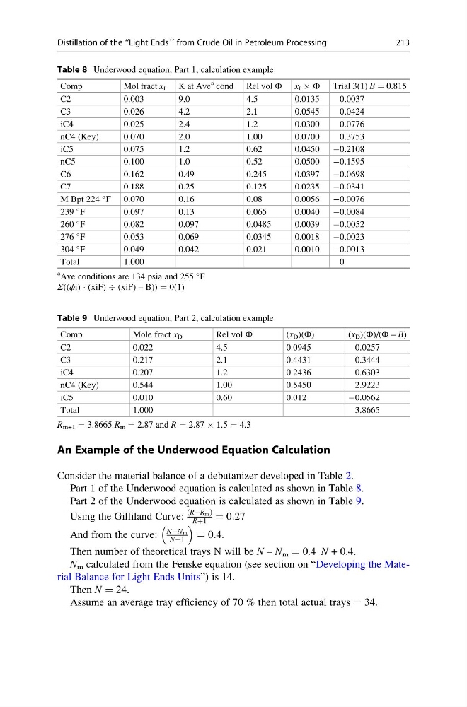
Part 1 of the Underwood equation is calculated as shown in Table 8.
Part 2 of the Underwood equation is calculated as shown in Table 9.
Using the Gilliland Curve:
RÀR m
ð
Þ
Rþ1 ¼ 0:27
And from the curve:
NÀN m
Nþ1
¼ 0:4:
Then number of theoretical trays N will be N – N m = 0.4 N + 0.4.
N m calculated from the Fenske equation (see section on “Developing the Material Balance for Light Ends Units”) is 14.
Then N = 24.
Assume an average tray efficiency of 70 % then total actual trays = 34.
Table 8 Underwood equation, Part 1, calculation example
Comp
Mol fract x f K at Ave
a cond Rel vol Ф x f Â Ф Trial 3(1) B = 0.815
C2
0.003
9.0
4.5
0.0135
0.0037
C3
0.026
4.2
2.1
0.0545
0.0424
iC4
0.025
2.4
1.2
0.0300
0.0776
nC4 (Key)
0.070
2.0
1.00
0.0700
0.3753
iC5
0.075
1.2
0.62
0.0450 À0.2108
nC5
0.100
1.0
0.52
0.0500 À0.1595
C6
0.162
0.49
0.245
0.0397 À0.0698
C7
0.188
0.25
0.125
0.0235 À0.0341
M Bpt 224
F 0.070
0.16
0.08
0.0056 À0.0076
239
F
0.097
0.13
0.065
0.0040 À0.0084
260
F
0.082
0.097
0.0485
0.0039 À0.0052
276
F
0.053
0.069
0.0345
0.0018 À0.0023
304
F
0.049
0.042
0.021
0.0010 À0.0013
Total
1.000
0
a
Ave conditions are 134 psia and 255
F
Σ((ϕi) Á (xiF) Ä (xiF) – B)) = 0(1)
Table 9 Underwood equation, Part 2, calculation example
Comp
Mole fract x D
Rel vol Ф
(x D )(Ф)
( x D )(Ф)/(Ф – B)
C2
0.022
4.5
0.0945
0.0257
C3
0.217
2.1
0.4431
0.3444
iC4
0.207
1.2
0.2436
0.6303
nC4 (Key)
0.544
1.00
0.5450
2.9223
iC5
0.010
0.60
0.012
À0.0562
Total
1.000
3.8665
R m+1 = 3.8665 R m = 2.87 and R = 2.87 Â 1.5 = 4.3
Distillation of the ‘‘Light Ends´´ from Crude Oil in Petroleum Processing
213
Consider the material balance of a debutanizer developed in Table 2.
Part 1 of the Underwood equation is calculated as shown in Table 8.
Part 2 of the Underwood equation is calculated as shown in Table 9.
Using the Gilliland Curve:
RÀR m
ð
Þ
Rþ1 ¼ 0:27
And from the curve:
NÀN m
Nþ1
¼ 0:4:
Then number of theoretical trays N will be N – N m = 0.4 N + 0.4.
N m calculated from the Fenske equation (see section on “Developing the Material Balance for Light Ends Units”) is 14.
Then N = 24.
Assume an average tray efficiency of 70 % then total actual trays = 34.
Table 8 Underwood equation, Part 1, calculation example
Comp
Mol fract x f K at Ave
a cond Rel vol Ф x f Â Ф Trial 3(1) B = 0.815
C2
0.003
9.0
4.5
0.0135
0.0037
C3
0.026
4.2
2.1
0.0545
0.0424
iC4
0.025
2.4
1.2
0.0300
0.0776
nC4 (Key)
0.070
2.0
1.00
0.0700
0.3753
iC5
0.075
1.2
0.62
0.0450 À0.2108
nC5
0.100
1.0
0.52
0.0500 À0.1595
C6
0.162
0.49
0.245
0.0397 À0.0698
C7
0.188
0.25
0.125
0.0235 À0.0341
M Bpt 224
F 0.070
0.16
0.08
0.0056 À0.0076
239
F
0.097
0.13
0.065
0.0040 À0.0084
260
F
0.082
0.097
0.0485
0.0039 À0.0052
276
F
0.053
0.069
0.0345
0.0018 À0.0023
304
F
0.049
0.042
0.021
0.0010 À0.0013
Total
1.000
0
a
Ave conditions are 134 psia and 255
F
Σ((ϕi) Á (xiF) Ä (xiF) – B)) = 0(1)
Table 9 Underwood equation, Part 2, calculation example
Comp
Mole fract x D
Rel vol Ф
(x D )(Ф)
( x D )(Ф)/(Ф – B)
C2
0.022
4.5
0.0945
0.0257
C3
0.217
2.1
0.4431
0.3444
iC4
0.207
1.2
0.2436
0.6303
nC4 (Key)
0.544
1.00
0.5450
2.9223
iC5
0.010
0.60
0.012
À0.0562
Total
1.000
3.8665
R m+1 = 3.8665 R m = 2.87 and R = 2.87 Â 1.5 = 4.3
Distillation of the ‘‘Light Ends´´ from Crude Oil in Petroleum Processing
213