

other side, using these functionals within relativistic many-body perturbation theory
allows effectively to take into account the second –order atomic perturbation theory
(fourth-order QED perturbation theory) corrections. In our work the corresponding
functionals of Refs. [65, 66] have been used. As a result one can get the optimal
perturbation theory one-electron basis. In concrete calculations it is sufficient to use
more simplified procedure, which is reduced to the functional minimization using
the variation of the correlation potential parameter b in Eq. (17).
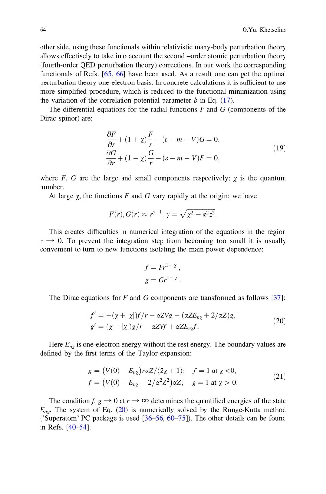
The differential equations for the radial functions F and G (components of the
Dirac spinor) are:
@F
@r
þ 1 þ v
ð
Þ
F
r
À e þ m À V
ð
Þ G ¼ 0;
@G
@r
þ 1 À v
ð
Þ
G
r
þ e À m À V
ð
Þ F ¼ 0;
ð19Þ
where F, G are the large and small components respectively; χ is the quantum
number.
At large χ, the functions F and G vary rapidly at the origin; we have
F r
ð Þ; G r
ð Þ % r
cÀ1
; c ¼
ffiffiffiffiffiffiffiffiffiffiffiffiffiffiffiffiffiffi ffi
v 2 À a 2 z 2
p
:
This creates difficulties in numerical integration of the equations in the region
r → 0. To prevent the integration step from becoming too small it is usually
convenient to turn to new functions isolating the main power dependence:
f ¼ Fr
1À v
j j
;
g ¼ Gr
1À v
j j
:
The Dirac equations for F and G components are transformed as follows [37]:
f
0
¼ Àðv þ jvjÞf =r À aZVg À ðaZE nv þ 2=aZÞg;
g
0
¼ ðv À jvjÞg=r À aZVf þ aZE nv f :
ð20Þ
Here E nχ is one-electron energy without the rest energy. The boundary values are
defined by the first terms of the Taylor expansion:
g ¼ V 0
ð Þ À E nv
À
Á
raZ= 2v þ 1
ð
Þ; f ¼ 1 at v\0;
f ¼ V 0
ð Þ À E nv À 2
a
2 Z
2
À
Á aZ; g ¼ 1 at v [ 0:
ð21Þ
The condition f, g → 0 at r → ∞ determines the quantified energies of the state
E nχ . The system of Eq. (20) is numerically solved by the Runge-Kutta method
(‘Superatom’ PC package is used [36–56, 60–75]). The other details can be found
in Refs. [40–54].
64
O.Yu. Khetselius
allows effectively to take into account the second –order atomic perturbation theory
(fourth-order QED perturbation theory) corrections. In our work the corresponding
functionals of Refs. [65, 66] have been used. As a result one can get the optimal
perturbation theory one-electron basis. In concrete calculations it is sufficient to use
more simplified procedure, which is reduced to the functional minimization using
the variation of the correlation potential parameter b in Eq. (17).
The differential equations for the radial functions F and G (components of the
Dirac spinor) are:
@F
@r
þ 1 þ v
ð
Þ
F
r
À e þ m À V
ð
Þ G ¼ 0;
@G
@r
þ 1 À v
ð
Þ
G
r
þ e À m À V
ð
Þ F ¼ 0;
ð19Þ
where F, G are the large and small components respectively; χ is the quantum
number.
At large χ, the functions F and G vary rapidly at the origin; we have
F r
ð Þ; G r
ð Þ % r
cÀ1
; c ¼
ffiffiffiffiffiffiffiffiffiffiffiffiffiffiffiffiffiffi ffi
v 2 À a 2 z 2
p
:
This creates difficulties in numerical integration of the equations in the region
r → 0. To prevent the integration step from becoming too small it is usually
convenient to turn to new functions isolating the main power dependence:
f ¼ Fr
1À v
j j
;
g ¼ Gr
1À v
j j
:
The Dirac equations for F and G components are transformed as follows [37]:
f
0
¼ Àðv þ jvjÞf =r À aZVg À ðaZE nv þ 2=aZÞg;
g
0
¼ ðv À jvjÞg=r À aZVf þ aZE nv f :
ð20Þ
Here E nχ is one-electron energy without the rest energy. The boundary values are
defined by the first terms of the Taylor expansion:
g ¼ V 0
ð Þ À E nv
À
Á
raZ= 2v þ 1
ð
Þ; f ¼ 1 at v\0;
f ¼ V 0
ð Þ À E nv À 2
a
2 Z
2
À
Á aZ; g ¼ 1 at v [ 0:
ð21Þ
The condition f, g → 0 at r → ∞ determines the quantified energies of the state
E nχ . The system of Eq. (20) is numerically solved by the Runge-Kutta method
(‘Superatom’ PC package is used [36–56, 60–75]). The other details can be found
in Refs. [40–54].
64
O.Yu. Khetselius