

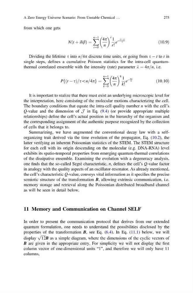
from which one gets
N t þ i hb
ð
Þ¼
X nÀ1
r¼0
4p
n
r 1
r!
e
À
ðtÀsÞ
s
ð10:9Þ
Dividing the lifetime s into n=4p discrete time units, or going from s À t to t in
single steps, defines a cumulative Poisson statistics for the intra-cell quantumthermal correlated ensemble with the intensity (rate) parameter k ¼ 4p=n, i.e.
P ðt À sÞ=s\n=4p
f
g ¼
X nÀ1
k¼0
4p
n
k 1
k!
e
À
4p
n
ð10:10Þ
It is important to realize that there must exist an underlying microscopic level for
the interpretation, here consisting of the molecular motions characterizing the cell.
The boundary conditions that equate the intra-cell quality number n with the cell’s
Q-value and the dimension of J in Eq. (9.4) (or provide appropriate multiple
relationships) define the cell’s actual position in the hierarchy of the organism and
the corresponding assignment of the authentic purpose recognized by the collection
of cells that it belongs to.
Summarizing, we have augmented the conventional decay law with a selforganizing trait derived via the time evolution of the propagator, Eq. (10.2), the
latter verifying an inherent Poissonian statistics of the STEM. The STEM structure
for each cell with its origin descending on the molecular (e.g. DNA-RNA) level
exhibits its spatio-temporal properties from emerging quantum-thermal correlations
of the dissipative ensemble. Examining the evolution with a degeneracy analysis,
one finds that the so-called Segrè characteristic, n, defines the cell’s Q-value factor
in analogy with the quality aspects of an oscillator-resonator. As already mentioned,
the cell’s characteristic Q-value, conveys vital information as it specifies the precise
semiotic structure of the transformation B, allowing extrinsic communication, i.e.
memory storage and retrieval along the Poissonian distributed broadband channel
as will be seen in detail below.
11 Memory and Communication on Channel SELF
In order to present the communication protocol that derives from our extended
quantum formulation, one needs to understand the possibilities disclosed by the
properties of the transformation B, see Eq. (6.4). In Eq. (11.1) below, we will
display
ffiffiffiffiffi
12
p B as a simple diagram, where the dimensions of the cyclic vectors of
B are given in the appropriate entry. For simplicity we will not display the first
column vector of one-dimensional units “1”, and therefore we will only have 11
columns,
A Zero Energy Universe Scenario: From Unstable Chemical …
275
N t þ i hb
ð
Þ¼
X nÀ1
r¼0
4p
n
r 1
r!
e
À
ðtÀsÞ
s
ð10:9Þ
Dividing the lifetime s into n=4p discrete time units, or going from s À t to t in
single steps, defines a cumulative Poisson statistics for the intra-cell quantumthermal correlated ensemble with the intensity (rate) parameter k ¼ 4p=n, i.e.
P ðt À sÞ=s\n=4p
f
g ¼
X nÀ1
k¼0
4p
n
k 1
k!
e
À
4p
n
ð10:10Þ
It is important to realize that there must exist an underlying microscopic level for
the interpretation, here consisting of the molecular motions characterizing the cell.
The boundary conditions that equate the intra-cell quality number n with the cell’s
Q-value and the dimension of J in Eq. (9.4) (or provide appropriate multiple
relationships) define the cell’s actual position in the hierarchy of the organism and
the corresponding assignment of the authentic purpose recognized by the collection
of cells that it belongs to.
Summarizing, we have augmented the conventional decay law with a selforganizing trait derived via the time evolution of the propagator, Eq. (10.2), the
latter verifying an inherent Poissonian statistics of the STEM. The STEM structure
for each cell with its origin descending on the molecular (e.g. DNA-RNA) level
exhibits its spatio-temporal properties from emerging quantum-thermal correlations
of the dissipative ensemble. Examining the evolution with a degeneracy analysis,
one finds that the so-called Segrè characteristic, n, defines the cell’s Q-value factor
in analogy with the quality aspects of an oscillator-resonator. As already mentioned,
the cell’s characteristic Q-value, conveys vital information as it specifies the precise
semiotic structure of the transformation B, allowing extrinsic communication, i.e.
memory storage and retrieval along the Poissonian distributed broadband channel
as will be seen in detail below.
11 Memory and Communication on Channel SELF
In order to present the communication protocol that derives from our extended
quantum formulation, one needs to understand the possibilities disclosed by the
properties of the transformation B, see Eq. (6.4). In Eq. (11.1) below, we will
display
ffiffiffiffiffi
12
p B as a simple diagram, where the dimensions of the cyclic vectors of
B are given in the appropriate entry. For simplicity we will not display the first
column vector of one-dimensional units “1”, and therefore we will only have 11
columns,
A Zero Energy Universe Scenario: From Unstable Chemical …
275