

G t
ð Þ ¼ e
ÀiP
t
s ; G R xs
ð Þ ¼ xsI À P
ð
Þ
À1
ð10:1Þ
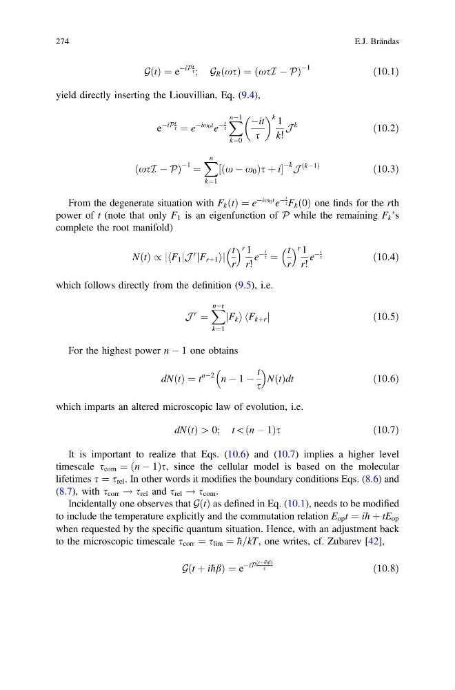
yield directly inserting the Liouvillian, Eq. (9.4),
e
ÀiP
t
s ¼ e
Àix 0 t e
À
t
s
X nÀ1
k¼0
Àit
s
k 1
k!
J
k
ð10:2Þ
xsI À P
ð
Þ
À1 ¼
X n
k¼1
x À x 0
ð
Þ s þ i
½
Àk J
ðkÀ1Þ
ð10:3Þ
From the degenerate situation with F k t
ð Þ ¼ e
Àix 0 t e
À
t
s F k 0
ð Þ one finds for the rth
power of t (note that only F 1 is an eigenfunction of P while the remaining F k ’s
complete the root manifold)
N t
ð Þ / F 1
h j
j
J
r F rþ1
j
ij
t
r
r 1
r!
e
À
t
s ¼
t
r
r 1
r!
e
À
t
s
ð10:4Þ
which follows directly from the definition (9.5), i.e.
J
r
¼
X nÀr
k¼1
F k
j i F kþr
h
j
ð10:5Þ
For the highest power n À 1 one obtains
dNðtÞ ¼ t
nÀ2 n À 1 À
t
s
N t
ð Þdt
ð10:6Þ
which imparts an altered microscopic law of evolution, i.e.
dN t
ð Þ [ 0; t\ n À 1
ð
Þs
ð10:7Þ
It is important to realize that Eqs. (10.6) and (10.7) implies a higher level
timescale s com ¼ ðn À 1Þs, since the cellular model is based on the molecular
lifetimes s ¼ s rel . In other words it modifies the boundary conditions Eqs. (8.6) and
(8.7), with s corr ! s rel and s rel ! s com .
Incidentally one observes that GðtÞ as defined in Eq. (10.1), needs to be modified
to include the temperature explicitly and the commutation relation E op t ¼ i h þ tE op
when requested by the specific quantum situation. Hence, with an adjustment back
to the microscopic timescale s corr ¼ s lim ¼ h=kT, one writes, cf. Zubarev [42],
G t þ i hb
ð
Þ¼e
ÀiP
tþi hb
ð
Þ
s
ð10:8Þ
274
E.J. Brändas
ð Þ ¼ e
ÀiP
t
s ; G R xs
ð Þ ¼ xsI À P
ð
Þ
À1
ð10:1Þ
yield directly inserting the Liouvillian, Eq. (9.4),
e
ÀiP
t
s ¼ e
Àix 0 t e
À
t
s
X nÀ1
k¼0
Àit
s
k 1
k!
J
k
ð10:2Þ
xsI À P
ð
Þ
À1 ¼
X n
k¼1
x À x 0
ð
Þ s þ i
½
Àk J
ðkÀ1Þ
ð10:3Þ
From the degenerate situation with F k t
ð Þ ¼ e
Àix 0 t e
À
t
s F k 0
ð Þ one finds for the rth
power of t (note that only F 1 is an eigenfunction of P while the remaining F k ’s
complete the root manifold)
N t
ð Þ / F 1
h j
j
J
r F rþ1
j
ij
t
r
r 1
r!
e
À
t
s ¼
t
r
r 1
r!
e
À
t
s
ð10:4Þ
which follows directly from the definition (9.5), i.e.
J
r
¼
X nÀr
k¼1
F k
j i F kþr
h
j
ð10:5Þ
For the highest power n À 1 one obtains
dNðtÞ ¼ t
nÀ2 n À 1 À
t
s
N t
ð Þdt
ð10:6Þ
which imparts an altered microscopic law of evolution, i.e.
dN t
ð Þ [ 0; t\ n À 1
ð
Þs
ð10:7Þ
It is important to realize that Eqs. (10.6) and (10.7) implies a higher level
timescale s com ¼ ðn À 1Þs, since the cellular model is based on the molecular
lifetimes s ¼ s rel . In other words it modifies the boundary conditions Eqs. (8.6) and
(8.7), with s corr ! s rel and s rel ! s com .
Incidentally one observes that GðtÞ as defined in Eq. (10.1), needs to be modified
to include the temperature explicitly and the commutation relation E op t ¼ i h þ tE op
when requested by the specific quantum situation. Hence, with an adjustment back
to the microscopic timescale s corr ¼ s lim ¼ h=kT, one writes, cf. Zubarev [42],
G t þ i hb
ð
Þ¼e
ÀiP
tþi hb
ð
Þ
s
ð10:8Þ
274
E.J. Brändas