difference. It is well known that the functions of a state for two nuclear potentials
differ significantly in the important region. Calculation of the potentials, their
derivatives, matrix elements is reduced to solving the single system (in fact 1D
procedure) of the differential equations (c.f. [45–54, 60, 70–72]).
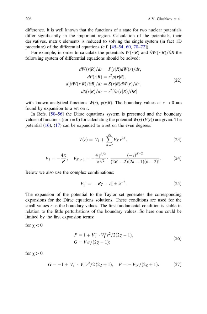
For example, in order to calculate the potentials W rjR
ð Þ and @W rjR
ð Þ=@R the
following system of differential equations should be solved:
dW rjR
ð Þ=dr ¼ P rjR
ð ÞdW r
ð Þ=dr;
dP rjR
ð Þ ¼ r
2
q rjR
ð Þ;
d½@W rjR
ð Þ=@RŠ=dr ¼ S rjR
ð ÞdW r
ð Þ=dr;
dS rjR
ð Þ=dr ¼ r
2
½@r rjR
ð Þ=@RŠ
ð22Þ
with known analytical functions W(r), ρ(r|R). The boundary values at r ! 0 are
found by expansion to a set on r.
In Refs. [50–56] the Dirac equations system is presented and the boundary
values of functions (for r = 0) for calculating the potential W(r) (V(r)) are given. The
potential (16), (17) can be expanded to a set on the even degrees:
V r
ð Þ ¼ V 1 þ
X 1
K¼2
V K r
2K
;
ð23Þ
V 1 ¼ À
4p
R
; V K [ 1 ¼ À
4 c
3=2
p 1=2 Á
Àc
ð Þ
KÀ2
2K À 2
ð
Þ2k À 1
ð
Þ k À 2
ð
Þ!
:
ð24Þ
Below we also use the complex combinations:
V
Æ
1 ¼ À Rc À in Æ ~ a
À2
:
ð25Þ
The expansion of the potential to the Taylor set generates the corresponding
expansions for the Dirac equations solutions. These conditions are used for the
small values r as the boundary values. The first fundamental condition is stable in
relation to the little perturbations of the boundary values. So here one could be
limited by the first expansion terms:
for χ < 0
F ¼ 1 þ V
À
1 Á V
þ
1 r
2
=2 2v À 1
ð
Þ;
G ¼ V 1 r= 2v À 1
ð
Þ;
ð26Þ
for χ > 0
G ¼ À1 þ V
À
1 Á V
þ
1 r
2
=2 2v þ 1
ð
Þ; F ¼ À V 1 r= 2v þ 1
ð
Þ:
ð27Þ
206
A.V. Glushkov et al.