

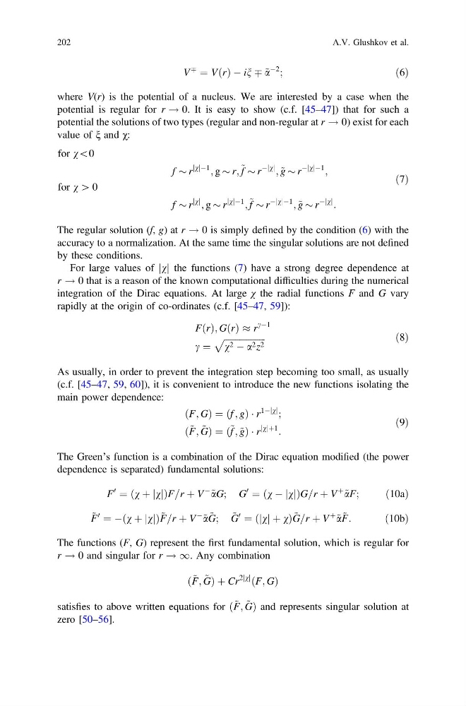
V
Ç
¼ VðrÞ À in Ç ~ a
À2
;
ð6Þ
where V(r) is the potential of a nucleus. We are interested by a case when the
potential is regular for r ! 0. It is easy to show (c.f. [45–47]) that for such a
potential the solutions of two types (regular and non-regular at r ! 0) exist for each
value of ξ and χ:
for v\0
f $ r
v
j jÀ1
; g $ r; ~ f $ r
À v
j j
; ~ g $ r
À v
j jÀ1
;
for v [ 0
f $ r
v
j j
; g $ r
v
j jÀ1
; ~ f $ r
À v
j jÀ1
; ~ g $ r
À v
j j
:
ð7Þ
The regular solution (f, g) at r ! 0 is simply defined by the condition (6) with the
accuracy to a normalization. At the same time the singular solutions are not defined
by these conditions.
For large values of v
j j the functions (7) have a strong degree dependence at
r ! 0 that is a reason of the known computational difficulties during the numerical
integration of the Dirac equations. At large χ the radial functions F and G vary
rapidly at the origin of co-ordinates (c.f. [45–47, 59]):
FðrÞ; GðrÞ % r
cÀ1
c ¼
ffiffiffiffiffiffiffiffiffiffiffiffiffiffiffiffiffiffi ffi
v 2 À a 2 z 2
p
ð8Þ
As usually, in order to prevent the integration step becoming too small, as usually
(c.f. [45–47, 59, 60]), it is convenient to introduce the new functions isolating the
main power dependence:
ðF; GÞ ¼ ðf ; gÞ Á r
1À v
j j
;
ð ~
F; ~
GÞ ¼ ð ~ f ; ~ gÞ Á r
v
j jþ1
:
ð9Þ
The Green’s function is a combination of the Dirac equation modified (the power
dependence is separated) fundamental solutions:
F
0
¼ ðv þ v
j jÞF=r þ V
À
~ aG; G
0
¼ ðv À v
j jÞG=r þ V
þ
~ aF;
ð10aÞ
~
F
0
¼ Àðv þ v
j jÞ ~
F=r þ V
À
~ a ~
G; ~
G
0
¼ ð v
j j þ vÞ ~
G=r þ V
þ
~ a ~
F:
ð10bÞ
The functions (F, G) represent the first fundamental solution, which is regular for
r ! 0 and singular for r ! 1. Any combination
ð ~
F; ~
GÞ þ Cr
2 v
j j
ðF; GÞ
satisfies to above written equations for ð ~
F; ~
GÞ and represents singular solution at
zero [50–56].
202
A.V. Glushkov et al.
Ç
¼ VðrÞ À in Ç ~ a
À2
;
ð6Þ
where V(r) is the potential of a nucleus. We are interested by a case when the
potential is regular for r ! 0. It is easy to show (c.f. [45–47]) that for such a
potential the solutions of two types (regular and non-regular at r ! 0) exist for each
value of ξ and χ:
for v\0
f $ r
v
j jÀ1
; g $ r; ~ f $ r
À v
j j
; ~ g $ r
À v
j jÀ1
;
for v [ 0
f $ r
v
j j
; g $ r
v
j jÀ1
; ~ f $ r
À v
j jÀ1
; ~ g $ r
À v
j j
:
ð7Þ
The regular solution (f, g) at r ! 0 is simply defined by the condition (6) with the
accuracy to a normalization. At the same time the singular solutions are not defined
by these conditions.
For large values of v
j j the functions (7) have a strong degree dependence at
r ! 0 that is a reason of the known computational difficulties during the numerical
integration of the Dirac equations. At large χ the radial functions F and G vary
rapidly at the origin of co-ordinates (c.f. [45–47, 59]):
FðrÞ; GðrÞ % r
cÀ1
c ¼
ffiffiffiffiffiffiffiffiffiffiffiffiffiffiffiffiffiffi ffi
v 2 À a 2 z 2
p
ð8Þ
As usually, in order to prevent the integration step becoming too small, as usually
(c.f. [45–47, 59, 60]), it is convenient to introduce the new functions isolating the
main power dependence:
ðF; GÞ ¼ ðf ; gÞ Á r
1À v
j j
;
ð ~
F; ~
GÞ ¼ ð ~ f ; ~ gÞ Á r
v
j jþ1
:
ð9Þ
The Green’s function is a combination of the Dirac equation modified (the power
dependence is separated) fundamental solutions:
F
0
¼ ðv þ v
j jÞF=r þ V
À
~ aG; G
0
¼ ðv À v
j jÞG=r þ V
þ
~ aF;
ð10aÞ
~
F
0
¼ Àðv þ v
j jÞ ~
F=r þ V
À
~ a ~
G; ~
G
0
¼ ð v
j j þ vÞ ~
G=r þ V
þ
~ a ~
F:
ð10bÞ
The functions (F, G) represent the first fundamental solution, which is regular for
r ! 0 and singular for r ! 1. Any combination
ð ~
F; ~
GÞ þ Cr
2 v
j j
ðF; GÞ
satisfies to above written equations for ð ~
F; ~
GÞ and represents singular solution at
zero [50–56].
202
A.V. Glushkov et al.