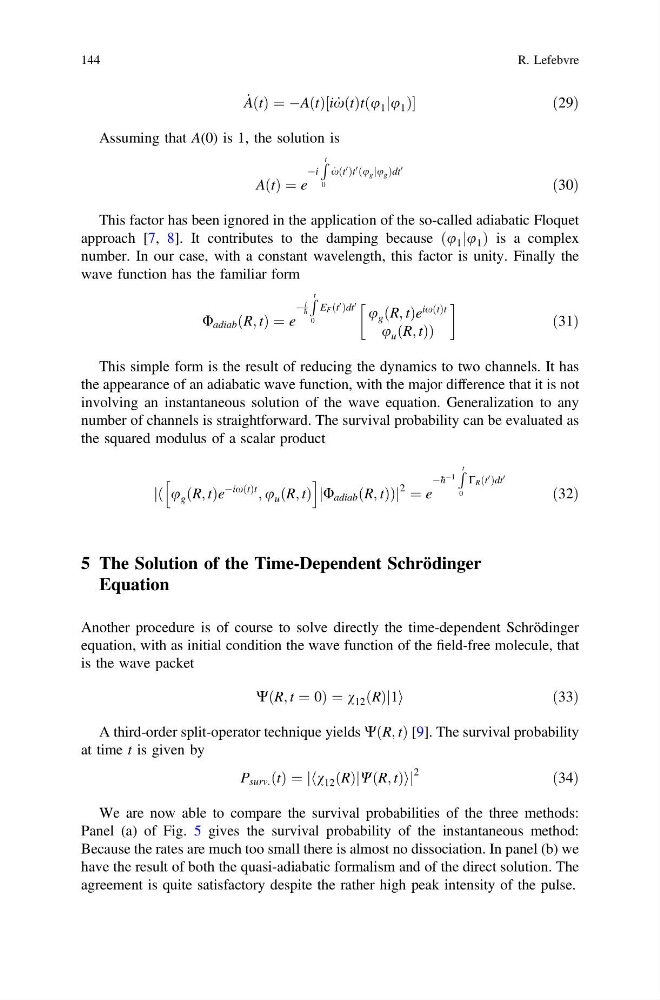
_
AðtÞ ¼ ÀAðtÞ½i _
xðtÞtðu 1 ju 1 ފ
ð29Þ
Assuming that A(0) is 1, the solution is
AðtÞ ¼ e
Ài
R t
0
_
xðt
0 Þt
0 ðu g ju g Þdt
0
ð30Þ
This factor has been ignored in the application of the so-called adiabatic Floquet
approach [7, 8]. It contributes to the damping because ðu 1 ju 1 Þ is a complex
number. In our case, with a constant wavelength, this factor is unity. Finally the
wave function has the familiar form
U adiab ðR; tÞ ¼ e
À
i
h
R t
0
E F ðt
0 Þdt
0
u g ðR; tÞe
ixðtÞt
u u ðR; tÞÞ
!
ð31Þ
This simple form is the result of reducing the dynamics to two channels. It has
the appearance of an adiabatic wave function, with the major difference that it is not
involving an instantaneous solution of the wave equation. Generalization to any
number of channels is straightforward. The survival probability can be evaluated as
the squared modulus of a scalar product
jð u g ðR; tÞe
ÀixðtÞt
; u u ðR; tÞ
h
i
jU adiab ðR; tÞÞj
2 ¼ e
À h
À1
R t
0
C R ðt
0 Þdt
0
ð32Þ
5 The Solution of the Time-Dependent Schrödinger
Equation
Another procedure is of course to solve directly the time-dependent Schrödinger
equation, with as initial condition the wave function of the field-free molecule, that
is the wave packet
WðR; t ¼ 0Þ ¼ v 12 ðRÞj1i
ð 33Þ
A third-order split-operator technique yields WðR; tÞ [9]. The survival probability
at time t is given by
P surv: ðtÞ ¼ jhv 12 ðRÞjWðR; tÞij
2
ð34Þ
We are now able to compare the survival probabilities of the three methods:
Panel (a) of Fig. 5 gives the survival probability of the instantaneous method:
Because the rates are much too small there is almost no dissociation. In panel (b) we
have the result of both the quasi-adiabatic formalism and of the direct solution. The
agreement is quite satisfactory despite the rather high peak intensity of the pulse.
144
R. Lefebvre