

6 Conclusion
The physical description of the quasi-adiabatic method is to let the system to be
exposed to a field with a frequency and an intensity corresponding to some point
along the curve describing the laser pulse and to let the field oscillate with these laser
parameters. This is repeated for the next point, and so on. This is to be distinguished
from the common adiabatic picture, with introduction of instantaneous eigenstates.
The failure of the latter method is that the assumption of a slow variation of the
parameters is not at all fulfilled for a field in the optical range. The quasi-adiabatic
procedure can be validated by the full solution of the time-dependent Schrödinger
equation in a case where there is no non-adiabatic contamination, because the resonance is well isolated from others for the range of parameters we have considered.
Acknowledgments I thank M. Desouter-Lecomte for providing the code for the wave packet
calculations and O. Atabek for useful discussions.
References
1. Born M, Fock V (1928) Z Phys 51:165
2. Kato T (1950) J Phys Soc Jpn 5:435
3. Messiah A (1962) Quantum Mechanics. North Holland, Amsterdam
4. Sarandy MS, Lidar DA (2005) Phys Rev A 71:012331
0
1 0
2 0
3 0
0.9994
0.9996
0.9998
1
0
1 0
2 0
3 0
0.4
0.6
0.8
1
Time (fs)
Survival Probability
(a)
(b)
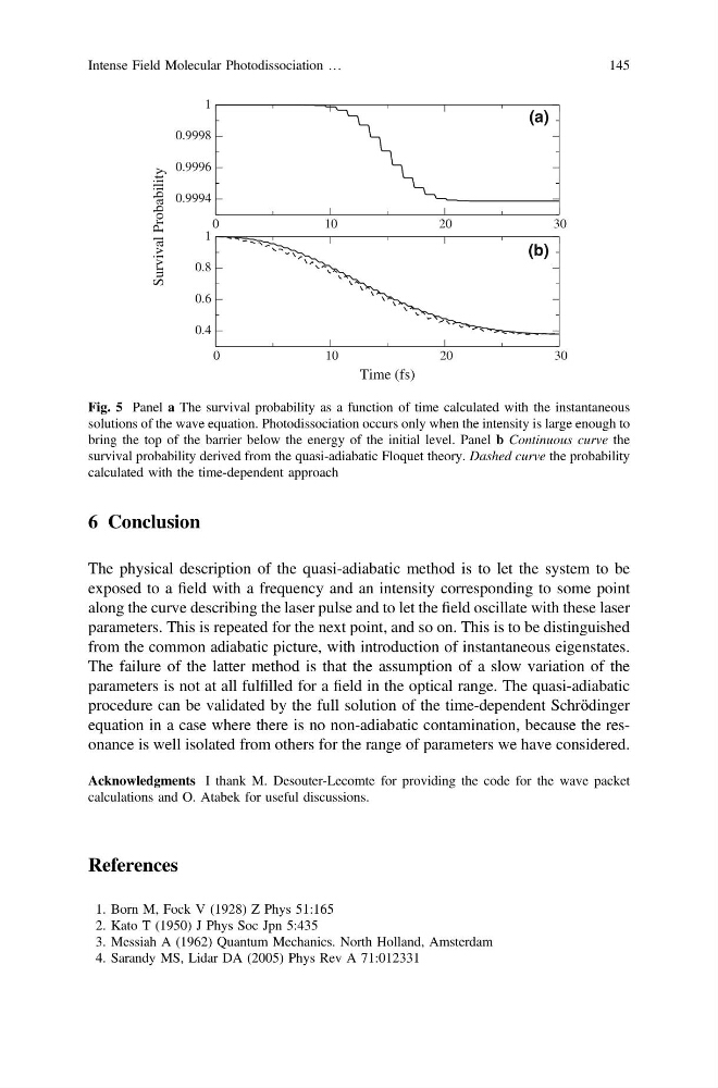
Fig. 5 Panel a The survival probability as a function of time calculated with the instantaneous
solutions of the wave equation. Photodissociation occurs only when the intensity is large enough to
bring the top of the barrier below the energy of the initial level. Panel b Continuous curve the
survival probability derived from the quasi-adiabatic Floquet theory. Dashed curve the probability
calculated with the time-dependent approach
Intense Field Molecular Photodissociation …
145
The physical description of the quasi-adiabatic method is to let the system to be
exposed to a field with a frequency and an intensity corresponding to some point
along the curve describing the laser pulse and to let the field oscillate with these laser
parameters. This is repeated for the next point, and so on. This is to be distinguished
from the common adiabatic picture, with introduction of instantaneous eigenstates.
The failure of the latter method is that the assumption of a slow variation of the
parameters is not at all fulfilled for a field in the optical range. The quasi-adiabatic
procedure can be validated by the full solution of the time-dependent Schrödinger
equation in a case where there is no non-adiabatic contamination, because the resonance is well isolated from others for the range of parameters we have considered.
Acknowledgments I thank M. Desouter-Lecomte for providing the code for the wave packet
calculations and O. Atabek for useful discussions.
References
1. Born M, Fock V (1928) Z Phys 51:165
2. Kato T (1950) J Phys Soc Jpn 5:435
3. Messiah A (1962) Quantum Mechanics. North Holland, Amsterdam
4. Sarandy MS, Lidar DA (2005) Phys Rev A 71:012331
0
1 0
2 0
3 0
0.9994
0.9996
0.9998
1
0
1 0
2 0
3 0
0.4
0.6
0.8
1
Time (fs)
Survival Probability
(a)
(b)
Fig. 5 Panel a The survival probability as a function of time calculated with the instantaneous
solutions of the wave equation. Photodissociation occurs only when the intensity is large enough to
bring the top of the barrier below the energy of the initial level. Panel b Continuous curve the
survival probability derived from the quasi-adiabatic Floquet theory. Dashed curve the probability
calculated with the time-dependent approach
Intense Field Molecular Photodissociation …
145