

in addition highlight areas where thin horizontal
resistors are present.
In Fig. 20.22 resistivity maps (R h and R v ), and
anisotropy map created from unconstrained inversion
of 3D CSEM data, are shown. All maps are calculated
with a 1,000 m wide window centred on the Base
Cretaceous unconformity. The horizontal resistivity
map shows the regional resistivity trend in the data.
This is also the case for the vertical resistivity map, but
in addition two distinct anomalies appear. One is at the
location of the Havis discovery, and the other (Lead 1)
is southeast of Well 7219/9-1. Only a very weak
anomaly is associated with the Skrugard discovery
well 7220/8-1.
Figure 20.22c shows the apparent anisotropy. In
this map three main anomalies are clearly observed.
Havis and Lead 1 are already identified in the vertical
resistivity map. In addition the Skrugard discovery is
now identified as a strong anomaly. The Skrugard and
Havis discoveries are located in rotated fault-blocks in
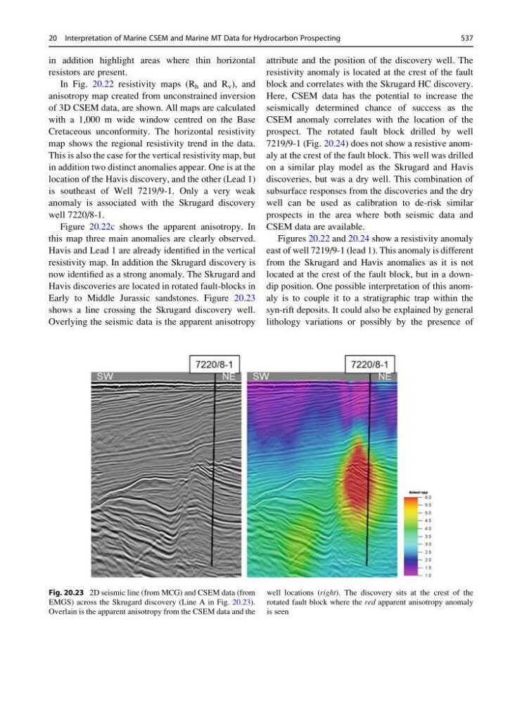
Early to Middle Jurassic sandstones. Figure 20.23
shows a line crossing the Skrugard discovery well.
Overlying the seismic data is the apparent anisotropy
attribute and the position of the discovery well. The
resistivity anomaly is located at the crest of the fault
block and correlates with the Skrugard HC discovery.
Here, CSEM data has the potential to increase the
seismically determined chance of success as the
CSEM anomaly correlates with the location of the
prospect. The rotated fault block drilled by well
7219/9-1 (Fig. 20.24) does not show a resistive anomaly at the crest of the fault block. This well was drilled
on a similar play model as the Skrugard and Havis
discoveries, but was a dry well. This combination of
subsurface responses from the discoveries and the dry
well can be used as calibration to de-risk similar
prospects in the area where both seismic data and
CSEM data are available.
Figures 20.22 and 20.24 show a resistivity anomaly
east of well 7219/9-1 (lead 1). This anomaly is different
from the Skrugard and Havis anomalies as it is not
located at the crest of the fault block, but in a downdip position. One possible interpretation of this anomaly is to couple it to a stratigraphic trap within the
syn-rift deposits. It could also be explained by general
lithology variations or possibly by the presence of
Fig. 20.23 2D seismic line (from MCG) and CSEM data (from
EMGS) across the Skrugard discovery (Line A in Fig. 20.23).
Overlain is the apparent anisotropy from the CSEM data and the
well locations (right). The discovery sits at the crest of the
rotated fault block where the red apparent anisotropy anomaly
is seen
20 Interpretation of Marine CSEM and Marine MT Data for Hydrocarbon Prospecting
537
resistors are present.
In Fig. 20.22 resistivity maps (R h and R v ), and
anisotropy map created from unconstrained inversion
of 3D CSEM data, are shown. All maps are calculated
with a 1,000 m wide window centred on the Base
Cretaceous unconformity. The horizontal resistivity
map shows the regional resistivity trend in the data.
This is also the case for the vertical resistivity map, but
in addition two distinct anomalies appear. One is at the
location of the Havis discovery, and the other (Lead 1)
is southeast of Well 7219/9-1. Only a very weak
anomaly is associated with the Skrugard discovery
well 7220/8-1.
Figure 20.22c shows the apparent anisotropy. In
this map three main anomalies are clearly observed.
Havis and Lead 1 are already identified in the vertical
resistivity map. In addition the Skrugard discovery is
now identified as a strong anomaly. The Skrugard and
Havis discoveries are located in rotated fault-blocks in
Early to Middle Jurassic sandstones. Figure 20.23
shows a line crossing the Skrugard discovery well.
Overlying the seismic data is the apparent anisotropy
attribute and the position of the discovery well. The
resistivity anomaly is located at the crest of the fault
block and correlates with the Skrugard HC discovery.
Here, CSEM data has the potential to increase the
seismically determined chance of success as the
CSEM anomaly correlates with the location of the
prospect. The rotated fault block drilled by well
7219/9-1 (Fig. 20.24) does not show a resistive anomaly at the crest of the fault block. This well was drilled
on a similar play model as the Skrugard and Havis
discoveries, but was a dry well. This combination of
subsurface responses from the discoveries and the dry
well can be used as calibration to de-risk similar
prospects in the area where both seismic data and
CSEM data are available.
Figures 20.22 and 20.24 show a resistivity anomaly
east of well 7219/9-1 (lead 1). This anomaly is different
from the Skrugard and Havis anomalies as it is not
located at the crest of the fault block, but in a downdip position. One possible interpretation of this anomaly is to couple it to a stratigraphic trap within the
syn-rift deposits. It could also be explained by general
lithology variations or possibly by the presence of
Fig. 20.23 2D seismic line (from MCG) and CSEM data (from
EMGS) across the Skrugard discovery (Line A in Fig. 20.23).
Overlain is the apparent anisotropy from the CSEM data and the
well locations (right). The discovery sits at the crest of the
rotated fault block where the red apparent anisotropy anomaly
is seen
20 Interpretation of Marine CSEM and Marine MT Data for Hydrocarbon Prospecting
537