

prospects that can be detected should be within size for
a commercial discovery in the region. In the Barents
Sea such CSEM grids are actively used by oil
companies for licencing round exploration, and also
in some cases for drilling decisions.
Identifying prospective areas based on CSEM data
alone is challenging. Also 2D seismic data will have
its limitations due to coarse coverage and possible
imaging problems. However, the combination of the
two data types can be a powerful tool in exploration.
Seismic data is used for geological understanding,
structural mapping, play development, and to map
prospect outlines. Resistivity trends and anomalies
observed in the CSEM data can be better understood
when integrated with seismic data. In this way, lack of
3D seismic information can to some extent be
compensated for by the 3D resistivity information
obtained from CSEM data. The EM data can also, in
some cases, carry structural and geometric information that can guide the interpretation between the seismic 2D lines. Once a prospective area has been
identified on seismic, 3D CSEM data can be used to
upgrade or downgrade prospects. CSEM data can also
generate new leads and prospects not yet identified by
the seismic. Especially stratigraphic traps are often
difficult to identify on seismic data.
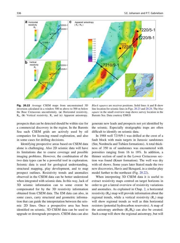
In 1988 well 7219/9-1 was drilled at the crest of a
fault block with main targets in Jurassic sandstones
(Stø, Nordmela and Tuba ˚en formations). A total thickness of 350 m of sandstones was encountered with
porosities ranging from 16 to 18%. In addition, a
thinner section of sand in the Lower Cretaceous section was found (Knurr formation). The well was dry
with oil shows. Some years later Statoil made the two
new discoveries, Havis and Skrugard, in a similar play
model further to the northeast (Fig. 20.22).
When interpreting 3D CSEM data it is useful to
extract resistivity maps centred on target horizons in
order to get a lateral overview of resistivity variations
and anomalies. As explained in Chap. 2, a horizontal
resistivity (R h ) map will provide information about the
regional trends, while a vertical resistivity (R v ) map
will show regional trends as well as thin horizontal
resistors (potential hydrocarbon reservoirs). A map of
the anisotropy attribute (R v /R h ) can also be created.
Such a map will show the regional anisotropy, but will
Fig. 20.22 Average CSEM maps from unconstrained 3D
inversion calculated in a window 500 m above to 500 m below
the Base Cretaceous unconformity. (a) Horizontal resistivity,
R h , (b) Vertical resistivity, R v and (c) Apparent anisotropy.
Black squares are receiver positions. Solid lines A and B show
line location for seismic lines in Figs. 20.23 and 20.24. The blue
square in the small overview map shows survey location in the
Barents Sea. Data courtesy EMGS
536
S.E. Johansen and P.T. Gabrielsen
a commercial discovery in the region. In the Barents
Sea such CSEM grids are actively used by oil
companies for licencing round exploration, and also
in some cases for drilling decisions.
Identifying prospective areas based on CSEM data
alone is challenging. Also 2D seismic data will have
its limitations due to coarse coverage and possible
imaging problems. However, the combination of the
two data types can be a powerful tool in exploration.
Seismic data is used for geological understanding,
structural mapping, play development, and to map
prospect outlines. Resistivity trends and anomalies
observed in the CSEM data can be better understood
when integrated with seismic data. In this way, lack of
3D seismic information can to some extent be
compensated for by the 3D resistivity information
obtained from CSEM data. The EM data can also, in
some cases, carry structural and geometric information that can guide the interpretation between the seismic 2D lines. Once a prospective area has been
identified on seismic, 3D CSEM data can be used to
upgrade or downgrade prospects. CSEM data can also
generate new leads and prospects not yet identified by
the seismic. Especially stratigraphic traps are often
difficult to identify on seismic data.
In 1988 well 7219/9-1 was drilled at the crest of a
fault block with main targets in Jurassic sandstones
(Stø, Nordmela and Tuba ˚en formations). A total thickness of 350 m of sandstones was encountered with
porosities ranging from 16 to 18%. In addition, a
thinner section of sand in the Lower Cretaceous section was found (Knurr formation). The well was dry
with oil shows. Some years later Statoil made the two
new discoveries, Havis and Skrugard, in a similar play
model further to the northeast (Fig. 20.22).
When interpreting 3D CSEM data it is useful to
extract resistivity maps centred on target horizons in
order to get a lateral overview of resistivity variations
and anomalies. As explained in Chap. 2, a horizontal
resistivity (R h ) map will provide information about the
regional trends, while a vertical resistivity (R v ) map
will show regional trends as well as thin horizontal
resistors (potential hydrocarbon reservoirs). A map of
the anisotropy attribute (R v /R h ) can also be created.
Such a map will show the regional anisotropy, but will
Fig. 20.22 Average CSEM maps from unconstrained 3D
inversion calculated in a window 500 m above to 500 m below
the Base Cretaceous unconformity. (a) Horizontal resistivity,
R h , (b) Vertical resistivity, R v and (c) Apparent anisotropy.
Black squares are receiver positions. Solid lines A and B show
line location for seismic lines in Figs. 20.23 and 20.24. The blue
square in the small overview map shows survey location in the
Barents Sea. Data courtesy EMGS
536
S.E. Johansen and P.T. Gabrielsen