

deep water in the Gulf of Mexico. The trap is an
anticline structure with a well-known regional reservoir interval approximately 700 m below the mud line.
The prospect is covered by both 3D seismic and 3D
CSEM data.
A seismic amplitude anomaly defines the maximum extent of the prospect, and a seismic flat spot
defines a possible internal gas/fluid contact
(Fig. 20.20). One possible model explaining these
seismic observations is that the flat spot represents
the gas/oil contact, and that the seismic amplitude
anomaly below the flat spot is caused by presence of
oil in the reservoir.
From the 3D inverted CSEM data we see that a
resistive anomaly is consistent with the outline of the
seismic flat spot (Fig. 20.21). There is no CSEM
anomaly associated with the seismic anomaly below
the flat spot. The combined DHI observations are
interpreted to be due to variation in hydrocarbon saturation within the prospect. The crest of the structure
was interpreted to have high saturation gas as there is a
strong DHI indicator in both the seismic- and CSEM
data. The lower part of the structure was interpreted to
have low hydrocarbon saturation as there is no resistive anomaly associated with the seismic amplitude
anomaly.
This combined seismic and CSEM interpretation
was confirmed by a well showing high gas saturation
and good reservoir sand at the top of the structure
down to the flat spot. The same sand was also
identified in an appraisal well down-dip on the structure, but here the reservoir sandstone had low hydrocarbon saturation as predicted in the interpretation.
20.6 Barents Sea Case Study
This case study shows how the combination of 2D
seismic data and 3D CSEM data can be interpreted
and used in exploration. 3D CSEM data covers the
Johan Castberg field (Skrugard and Havis discoveries)
on the Polheim sub-platform in the Barents Sea
(Fig. 20.22). The survey also includes the exploration
well 7219/9-1 to the southwest of the field. The
Skrugard and Havis discoveries made in 2012 were
based on observations on 3D seismic data (double flat
10
4
10 3
10
2
10
1
10
0
0
0.1 0.2 0.3 0.4
0.4
0.5 0.6 0.7 0.8
0.8
0.9
1
1.0
0.5
0.0
Water saturation
Gas saturation
1.2
1.6
P-wave velocity (km/s)
V e lo c it y
Fizz gas
A r c h i e ’s
Seawater/gas in 50% porous sandstone
Resistivity ( m, log scale)
Ω
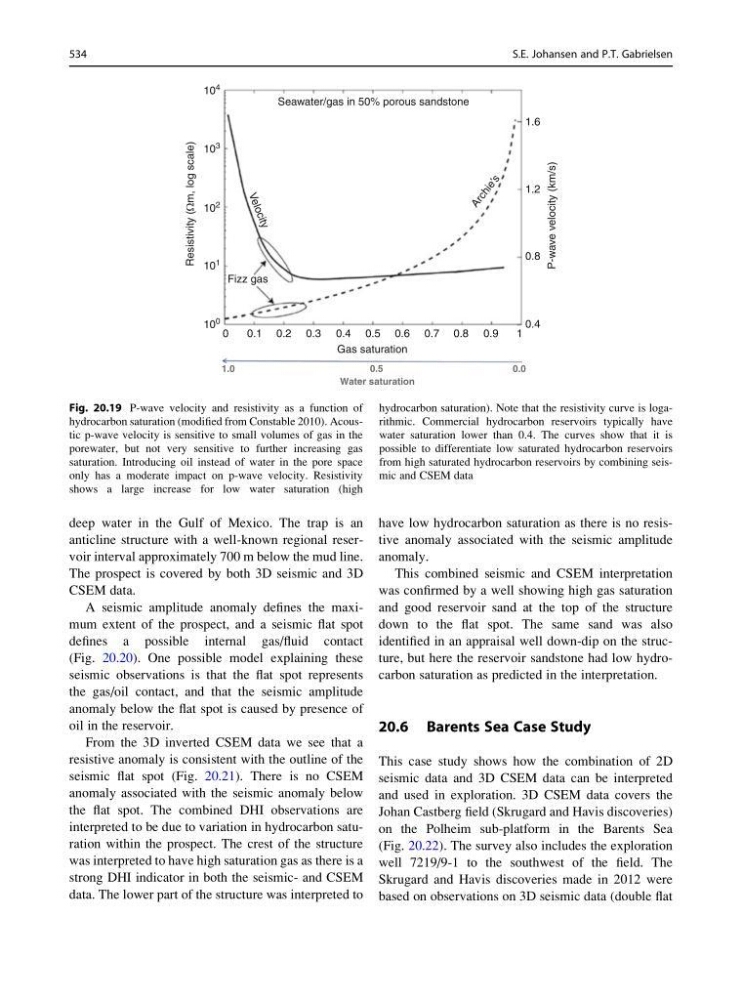
Fig. 20.19 P-wave velocity and resistivity as a function of
hydrocarbon saturation (modified from Constable 2010). Acoustic p-wave velocity is sensitive to small volumes of gas in the
porewater, but not very sensitive to further increasing gas
saturation. Introducing oil instead of water in the pore space
only has a moderate impact on p-wave velocity. Resistivity
shows a large increase for low water saturation (high
hydrocarbon saturation). Note that the resistivity curve is logarithmic. Commercial hydrocarbon reservoirs typically have
water saturation lower than 0.4. The curves show that it is
possible to differentiate low saturated hydrocarbon reservoirs
from high saturated hydrocarbon reservoirs by combining seismic and CSEM data
534
S.E. Johansen and P.T. Gabrielsen
anticline structure with a well-known regional reservoir interval approximately 700 m below the mud line.
The prospect is covered by both 3D seismic and 3D
CSEM data.
A seismic amplitude anomaly defines the maximum extent of the prospect, and a seismic flat spot
defines a possible internal gas/fluid contact
(Fig. 20.20). One possible model explaining these
seismic observations is that the flat spot represents
the gas/oil contact, and that the seismic amplitude
anomaly below the flat spot is caused by presence of
oil in the reservoir.
From the 3D inverted CSEM data we see that a
resistive anomaly is consistent with the outline of the
seismic flat spot (Fig. 20.21). There is no CSEM
anomaly associated with the seismic anomaly below
the flat spot. The combined DHI observations are
interpreted to be due to variation in hydrocarbon saturation within the prospect. The crest of the structure
was interpreted to have high saturation gas as there is a
strong DHI indicator in both the seismic- and CSEM
data. The lower part of the structure was interpreted to
have low hydrocarbon saturation as there is no resistive anomaly associated with the seismic amplitude
anomaly.
This combined seismic and CSEM interpretation
was confirmed by a well showing high gas saturation
and good reservoir sand at the top of the structure
down to the flat spot. The same sand was also
identified in an appraisal well down-dip on the structure, but here the reservoir sandstone had low hydrocarbon saturation as predicted in the interpretation.
20.6 Barents Sea Case Study
This case study shows how the combination of 2D
seismic data and 3D CSEM data can be interpreted
and used in exploration. 3D CSEM data covers the
Johan Castberg field (Skrugard and Havis discoveries)
on the Polheim sub-platform in the Barents Sea
(Fig. 20.22). The survey also includes the exploration
well 7219/9-1 to the southwest of the field. The
Skrugard and Havis discoveries made in 2012 were
based on observations on 3D seismic data (double flat
10
4
10 3
10
2
10
1
10
0
0
0.1 0.2 0.3 0.4
0.4
0.5 0.6 0.7 0.8
0.8
0.9
1
1.0
0.5
0.0
Water saturation
Gas saturation
1.2
1.6
P-wave velocity (km/s)
V e lo c it y
Fizz gas
A r c h i e ’s
Seawater/gas in 50% porous sandstone
Resistivity ( m, log scale)
Ω
Fig. 20.19 P-wave velocity and resistivity as a function of
hydrocarbon saturation (modified from Constable 2010). Acoustic p-wave velocity is sensitive to small volumes of gas in the
porewater, but not very sensitive to further increasing gas
saturation. Introducing oil instead of water in the pore space
only has a moderate impact on p-wave velocity. Resistivity
shows a large increase for low water saturation (high
hydrocarbon saturation). Note that the resistivity curve is logarithmic. Commercial hydrocarbon reservoirs typically have
water saturation lower than 0.4. The curves show that it is
possible to differentiate low saturated hydrocarbon reservoirs
from high saturated hydrocarbon reservoirs by combining seismic and CSEM data
534
S.E. Johansen and P.T. Gabrielsen