

for all receivers. This intermediate offset interval
records close to maximum difference in measured
magnitudes ON and OFF TWGP. Median normalised
magnitudes at 6.5 Æ 0.5 km offset for all receivers are
illustrated in Fig. 20.18, with data plotted at 3.25 km
offset halfway between source and receivers. Median
normalised magnitudes are around 1.0 south west of
TWGP (OFF), increase gradually up to 2.7 over the
apex of the HC accumulation (ON), and decrease
gradually down to 1.2 over the northwestern fringes
of the field. The gradual increase is caused by the fact
that both source and receiver must be above the target
to record maximum returned energy from the HC
accumulation. For TWGP this is the case only for a
narrow zone above the middle part of the HC accumulation. We also see that the western slope of the anomaly is steeper than the eastern. A likely explanation for
this is the asymmetric shape of the accumulation with
a fault termination at the western extension and a more
gradual eastward thinning as shown in Fig. 20.18.
There are no observations of high resistive strata or
structures that we know of, other than the TWGP,
which can explain the high resistivity values measured
by the survey. Due to extensive seismic surveying and
drilling in this part of the North Sea, the geology of the
area is very well known.
20.5 Gulf of Mexico Case Study
CSEM data and seismic data measure different Earth
properties. The CSEM method is sensitive to resistivity variations, while the seismic method is sensitive to
velocity and density variations. Both methods are
therefore indirectly sensitive to HC saturation in a
reservoir. The seismic method can normally see
deeper into the subsurface than the CSEM method. It
is always important to control that the measured
targets are well inside the detectability range for the
method used. Especially for the CSEM method sensitivity studies should always be performed to check if
the actual prospect is within reach of the method.
Seismic velocity will have a sharp decrease when
introducing even small amounts of gas in a water-filled
sandstone reservoir. Since oil has comparable
velocities to saline water the velocity effect is much
5.0
4.5
4.0
3.5
3.0
2.5
2.0
1.5
1.0
0.5
0.0
–0.5
0
1000
2000
3000
4000
5000
6000
7000 8000
9000 10000
1800
1600
1400
1200
1000
800
600
400
200
0
Normalized magnitudes
Source - Receiver Distance (m)
0.33 m
Ω
0.33 m
Ω
1.4 m
250 m
5 m
Ω
1.4 m
Ω
Ω
2 m
Ω
2 m
Ω
2 m
Ω
1 m
Ω
1 m
Ω
1.5 m
Ω
1.5 m
Ω
1.5 m
Ω
Ω
250 m
Ω
0.33 m
Ω
On-Reservoir Off-Reservoir
Depth below Sealevel (m)
Receiver
Model E
Model A
Model F
Model C
Model D
Model B
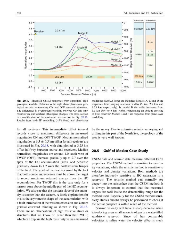
Fig. 20.17 Modelled CSEM responses from simplified Troll
geological models. Columns to the right show plane-layer geological models representing ON and OFF reservoir situations.
The differences in overburden resistivity between ON and OFF
reservoir are due to lateral lithological changes. The cross-section
is a modification of the east-west cross-section in Fig. 20.16.
Results from both 3D modelling (solid lines) and plane-layer
modelling (dashed lines) are included. Models A, C and D are
responses from varying reservoir widths (5 km, 2.5 km and
1.25 km respectively). In model B the width increases from
3.5 km (left) to 5 km (right), representing an oblique crossing
of Troll reservoir. Models E and F are responses from plane-layer
modelling
532
S.E. Johansen and P.T. Gabrielsen
records close to maximum difference in measured
magnitudes ON and OFF TWGP. Median normalised
magnitudes at 6.5 Æ 0.5 km offset for all receivers are
illustrated in Fig. 20.18, with data plotted at 3.25 km
offset halfway between source and receivers. Median
normalised magnitudes are around 1.0 south west of
TWGP (OFF), increase gradually up to 2.7 over the
apex of the HC accumulation (ON), and decrease
gradually down to 1.2 over the northwestern fringes
of the field. The gradual increase is caused by the fact
that both source and receiver must be above the target
to record maximum returned energy from the HC
accumulation. For TWGP this is the case only for a
narrow zone above the middle part of the HC accumulation. We also see that the western slope of the anomaly is steeper than the eastern. A likely explanation for
this is the asymmetric shape of the accumulation with
a fault termination at the western extension and a more
gradual eastward thinning as shown in Fig. 20.18.
There are no observations of high resistive strata or
structures that we know of, other than the TWGP,
which can explain the high resistivity values measured
by the survey. Due to extensive seismic surveying and
drilling in this part of the North Sea, the geology of the
area is very well known.
20.5 Gulf of Mexico Case Study
CSEM data and seismic data measure different Earth
properties. The CSEM method is sensitive to resistivity variations, while the seismic method is sensitive to
velocity and density variations. Both methods are
therefore indirectly sensitive to HC saturation in a
reservoir. The seismic method can normally see
deeper into the subsurface than the CSEM method. It
is always important to control that the measured
targets are well inside the detectability range for the
method used. Especially for the CSEM method sensitivity studies should always be performed to check if
the actual prospect is within reach of the method.
Seismic velocity will have a sharp decrease when
introducing even small amounts of gas in a water-filled
sandstone reservoir. Since oil has comparable
velocities to saline water the velocity effect is much
5.0
4.5
4.0
3.5
3.0
2.5
2.0
1.5
1.0
0.5
0.0
–0.5
0
1000
2000
3000
4000
5000
6000
7000 8000
9000 10000
1800
1600
1400
1200
1000
800
600
400
200
0
Normalized magnitudes
Source - Receiver Distance (m)
0.33 m
Ω
0.33 m
Ω
1.4 m
250 m
5 m
Ω
1.4 m
Ω
Ω
2 m
Ω
2 m
Ω
2 m
Ω
1 m
Ω
1 m
Ω
1.5 m
Ω
1.5 m
Ω
1.5 m
Ω
Ω
250 m
Ω
0.33 m
Ω
On-Reservoir Off-Reservoir
Depth below Sealevel (m)
Receiver
Model E
Model A
Model F
Model C
Model D
Model B
Fig. 20.17 Modelled CSEM responses from simplified Troll
geological models. Columns to the right show plane-layer geological models representing ON and OFF reservoir situations.
The differences in overburden resistivity between ON and OFF
reservoir are due to lateral lithological changes. The cross-section
is a modification of the east-west cross-section in Fig. 20.16.
Results from both 3D modelling (solid lines) and plane-layer
modelling (dashed lines) are included. Models A, C and D are
responses from varying reservoir widths (5 km, 2.5 km and
1.25 km respectively). In model B the width increases from
3.5 km (left) to 5 km (right), representing an oblique crossing
of Troll reservoir. Models E and F are responses from plane-layer
modelling
532
S.E. Johansen and P.T. Gabrielsen