

good indication of the main subsurface structures
(Fig. 20.15).
The apparent resistivity and impedance phase data
is used as input to inversion. The inversion transforms
the recorded data to a depth converted resistivity
model (see inversion section for details). MMT inversion algorithms only invert for the horizontal resistivity model as the natural source is dominantly a plane
horizontal field. The polarisation of the field is also
why the MMT method will see through horizontal
resistors such as basaltic layers. MMT data is used in
combination with CSEM data to map structures
beneath basaltic layers. MMT data can also be effective in mapping subsurface salt structures.
20.4 Troll Case Study
20.4.1 Troll West Gas Province
In this case study we present CSEM data across the
Troll West Gas Province (TWGP), offshore Norway.
The case is included as an example of pre-inversion
interpretation of marine CSEM data at receiver level.
The Troll Field complex is the largest gas discovery
on the Norwegian Continental Shelf, located in
300–360 m of water in the northeastern part of the
North Sea. The field is subdivided into three separate
compartments. Troll East is by far the largest and
contains two thirds of the HC reserves. For the
CSEM survey the much smaller TWGP was selected
(Fig. 20.16). The reservoir interval is Jurassic
sandstones (Sognefjord Fm.) with up to 160 m gas
column, and a thin oil leg at the base. HC-filled
sands show high average resistivities around
200–500 Ωm, and occur at a burial depth of about
1,400 m below sea level. Water-bearing Sognefjord
Fm. sands and overburden sediments show resistivities
in the 0.5–2 Ωm range. The TWGP was very well
suited for CSEM surveying, due to the high reservoir
resistivities, well defined field edges, the low and
relatively constant resistivities in the geological layers
above the reservoir (overburden), constant water
depth, smooth seafloor, and the moderate distribution
of the HC filled reservoir.
20.4.2 CSEM Forward Modelling
When interpreting CSEM data at receiver level the
CSEM response over the HC accumulation is compared with the CSEM response in a reference area
immediately outside the accumulation. It is also critical to understand CSEM responses from high resistivity bodies, other than the HC reservoir itself, which
can potentially generate significant responses.
Three dimensional modelling shows how the
CSEM response is affected by the geometry of the
reservoir and the effect of varying receiver layout
geometries. With the ultra-low frequencies (0.25 Hz)
used in CSEM sounding, it is the resistivity variations
in the illuminated subsurface that dominate the
response measured at the seafloor. All measured and
modelled CSEM responses are normalised to a reference case with no subsurface HC accumulation.
In this early case study, modelling had two main
goals; firstly, to establish the optimal survey location
and receiver geometry; and secondly, to quantify the
expected CSEM response from the subsurface HC
accumulation relative to that of a reference area outside the accumulation.
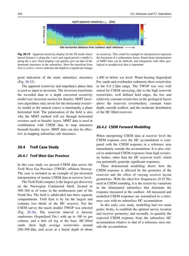
Fig. 20.15 Apparent resistivity display for the TE mode where
lateral distance is along the x-axis and signal period (~depth) is
along the y-axis. Such displays can quickly give an idea of the
dominant structures in the subsurface. Here the transition from
blue to yellow colours indicates the depth to a significant change
in resistivity. This could for example be interpreted to represent
the basement of a sedimentary basin. Stand-alone interpretation
of MMT data can be difficult, and integration with other geological or geophysical data is important
530
S.E. Johansen and P.T. Gabrielsen
(Fig. 20.15).
The apparent resistivity and impedance phase data
is used as input to inversion. The inversion transforms
the recorded data to a depth converted resistivity
model (see inversion section for details). MMT inversion algorithms only invert for the horizontal resistivity model as the natural source is dominantly a plane
horizontal field. The polarisation of the field is also
why the MMT method will see through horizontal
resistors such as basaltic layers. MMT data is used in
combination with CSEM data to map structures
beneath basaltic layers. MMT data can also be effective in mapping subsurface salt structures.
20.4 Troll Case Study
20.4.1 Troll West Gas Province
In this case study we present CSEM data across the
Troll West Gas Province (TWGP), offshore Norway.
The case is included as an example of pre-inversion
interpretation of marine CSEM data at receiver level.
The Troll Field complex is the largest gas discovery
on the Norwegian Continental Shelf, located in
300–360 m of water in the northeastern part of the
North Sea. The field is subdivided into three separate
compartments. Troll East is by far the largest and
contains two thirds of the HC reserves. For the
CSEM survey the much smaller TWGP was selected
(Fig. 20.16). The reservoir interval is Jurassic
sandstones (Sognefjord Fm.) with up to 160 m gas
column, and a thin oil leg at the base. HC-filled
sands show high average resistivities around
200–500 Ωm, and occur at a burial depth of about
1,400 m below sea level. Water-bearing Sognefjord
Fm. sands and overburden sediments show resistivities
in the 0.5–2 Ωm range. The TWGP was very well
suited for CSEM surveying, due to the high reservoir
resistivities, well defined field edges, the low and
relatively constant resistivities in the geological layers
above the reservoir (overburden), constant water
depth, smooth seafloor, and the moderate distribution
of the HC filled reservoir.
20.4.2 CSEM Forward Modelling
When interpreting CSEM data at receiver level the
CSEM response over the HC accumulation is compared with the CSEM response in a reference area
immediately outside the accumulation. It is also critical to understand CSEM responses from high resistivity bodies, other than the HC reservoir itself, which
can potentially generate significant responses.
Three dimensional modelling shows how the
CSEM response is affected by the geometry of the
reservoir and the effect of varying receiver layout
geometries. With the ultra-low frequencies (0.25 Hz)
used in CSEM sounding, it is the resistivity variations
in the illuminated subsurface that dominate the
response measured at the seafloor. All measured and
modelled CSEM responses are normalised to a reference case with no subsurface HC accumulation.
In this early case study, modelling had two main
goals; firstly, to establish the optimal survey location
and receiver geometry; and secondly, to quantify the
expected CSEM response from the subsurface HC
accumulation relative to that of a reference area outside the accumulation.
Fig. 20.15 Apparent resistivity display for the TE mode where
lateral distance is along the x-axis and signal period (~depth) is
along the y-axis. Such displays can quickly give an idea of the
dominant structures in the subsurface. Here the transition from
blue to yellow colours indicates the depth to a significant change
in resistivity. This could for example be interpreted to represent
the basement of a sedimentary basin. Stand-alone interpretation
of MMT data can be difficult, and integration with other geological or geophysical data is important
530
S.E. Johansen and P.T. Gabrielsen