

For the CSEM and MT methods the model m is the
Earth resistivity distribution that we are seeking and d
is the electric and magnetic field measured by the
receivers. However, we have several problems with
this equation. First of all we do not know the inverse
operator G
À1 . Second the operator G, which is forward
modelling based on Maxwell equations, is nonlinear.
Third the solution to our problem is ill posed. To
understand what ill posed means lets define a well
posed problem. A well posed problem means that a
solution exists. There is a unique solution (same data
measurement can only be explained by one model),
and the solution is stable (a small change in the model
creates a small change in the data measurement). If
one or more of these terms are broken we have an ill
posed problem. For CSEM and MT data our largest
challenge is the non-uniqueness. This means that
several resistivity models can create the same data
measurements. We can also be challenged with an
unstable solution. Because of the complexity of our
problem, we must do approximations and find the
solution in an iterative way. Instead of finding the
Earth resistivity model by using the inverse operator
G
À1 (which is unknown), we perform forward
modelling to simulate synthetic data based on a
given model:
d ¼ G m
ð Þ
The final inverted resistivity model is obtained by
finding a model, m, which gives the minimum difference between the synthetic data, d, and the measured
data using e.g. least square methods. These inversion
results will depend on the start model used, the
regularisation terms, a priori information applied to
constrain the results, and the number of dimensions
used in the forward modelling algorithm, G (1D, 2D or
3D). Due to the non-uniqueness of the solution,
performing inversion is just as much an interpretation
task as a data processing step.
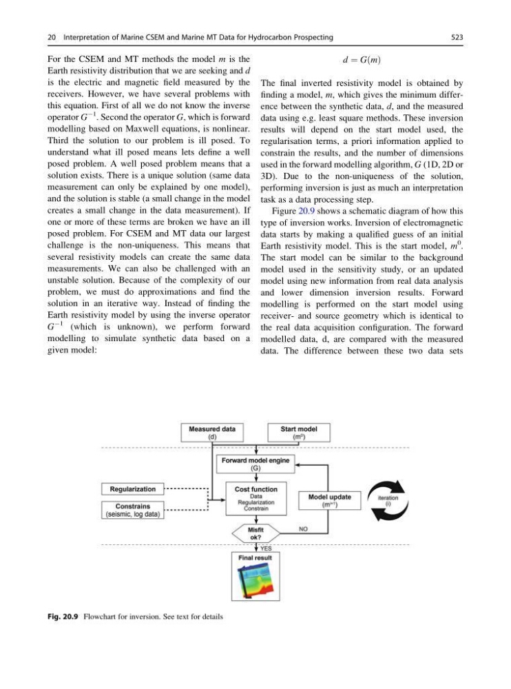
Figure 20.9 shows a schematic diagram of how this
type of inversion works. Inversion of electromagnetic
data starts by making a qualified guess of an initial
Earth resistivity model. This is the start model, m
0 .
The start model can be similar to the background
model used in the sensitivity study, or an updated
model using new information from real data analysis
and lower dimension inversion results. Forward
modelling is performed on the start model using
receiver- and source geometry which is identical to
the real data acquisition configuration. The forward
modelled data, d, are compared with the measured
data. The difference between these two data sets
Fig. 20.9 Flowchart for inversion. See text for details
20 Interpretation of Marine CSEM and Marine MT Data for Hydrocarbon Prospecting
523
Earth resistivity distribution that we are seeking and d
is the electric and magnetic field measured by the
receivers. However, we have several problems with
this equation. First of all we do not know the inverse
operator G
À1 . Second the operator G, which is forward
modelling based on Maxwell equations, is nonlinear.
Third the solution to our problem is ill posed. To
understand what ill posed means lets define a well
posed problem. A well posed problem means that a
solution exists. There is a unique solution (same data
measurement can only be explained by one model),
and the solution is stable (a small change in the model
creates a small change in the data measurement). If
one or more of these terms are broken we have an ill
posed problem. For CSEM and MT data our largest
challenge is the non-uniqueness. This means that
several resistivity models can create the same data
measurements. We can also be challenged with an
unstable solution. Because of the complexity of our
problem, we must do approximations and find the
solution in an iterative way. Instead of finding the
Earth resistivity model by using the inverse operator
G
À1 (which is unknown), we perform forward
modelling to simulate synthetic data based on a
given model:
d ¼ G m
ð Þ
The final inverted resistivity model is obtained by
finding a model, m, which gives the minimum difference between the synthetic data, d, and the measured
data using e.g. least square methods. These inversion
results will depend on the start model used, the
regularisation terms, a priori information applied to
constrain the results, and the number of dimensions
used in the forward modelling algorithm, G (1D, 2D or
3D). Due to the non-uniqueness of the solution,
performing inversion is just as much an interpretation
task as a data processing step.
Figure 20.9 shows a schematic diagram of how this
type of inversion works. Inversion of electromagnetic
data starts by making a qualified guess of an initial
Earth resistivity model. This is the start model, m
0 .
The start model can be similar to the background
model used in the sensitivity study, or an updated
model using new information from real data analysis
and lower dimension inversion results. Forward
modelling is performed on the start model using
receiver- and source geometry which is identical to
the real data acquisition configuration. The forward
modelled data, d, are compared with the measured
data. The difference between these two data sets
Fig. 20.9 Flowchart for inversion. See text for details
20 Interpretation of Marine CSEM and Marine MT Data for Hydrocarbon Prospecting
523