

20.2.5 Inversion
When we do electromagnetic acquisition (CSEM and
MT) the goal is to find the resistivity distribution in the
subsurface. However, what we measure is the electric
and magnetic fields recorded at the seabed. This is a
typical inverse problem as we seek a parameter (the
resistivity of the Earth) which we cannot directly
measure. In general terms an inversion problem can
be solved by finding the model m which explains the
measured data d using an operator G. The operator G
describes the explicit relationship between the model
(m) and the observed data (d):
m ¼ G
À1 d
ð Þ
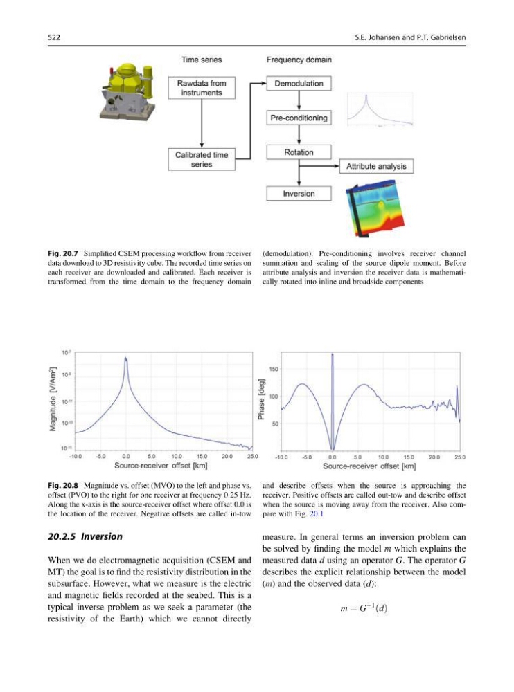
Fig. 20.7 Simplified CSEM processing workflow from receiver
data download to 3D resistivity cube. The recorded time series on
each receiver are downloaded and calibrated. Each receiver is
transformed from the time domain to the frequency domain
(demodulation). Pre-conditioning involves receiver channel
summation and scaling of the source dipole moment. Before
attribute analysis and inversion the receiver data is mathematically rotated into inline and broadside components
Fig. 20.8 Magnitude vs. offset (MVO) to the left and phase vs.
offset (PVO) to the right for one receiver at frequency 0.25 Hz.
Along the x-axis is the source-receiver offset where offset 0.0 is
the location of the receiver. Negative offsets are called in-tow
and describe offsets when the source is approaching the
receiver. Positive offsets are called out-tow and describe offset
when the source is moving away from the receiver. Also compare with Fig. 20.1
522
S.E. Johansen and P.T. Gabrielsen
When we do electromagnetic acquisition (CSEM and
MT) the goal is to find the resistivity distribution in the
subsurface. However, what we measure is the electric
and magnetic fields recorded at the seabed. This is a
typical inverse problem as we seek a parameter (the
resistivity of the Earth) which we cannot directly
measure. In general terms an inversion problem can
be solved by finding the model m which explains the
measured data d using an operator G. The operator G
describes the explicit relationship between the model
(m) and the observed data (d):
m ¼ G
À1 d
ð Þ
Fig. 20.7 Simplified CSEM processing workflow from receiver
data download to 3D resistivity cube. The recorded time series on
each receiver are downloaded and calibrated. Each receiver is
transformed from the time domain to the frequency domain
(demodulation). Pre-conditioning involves receiver channel
summation and scaling of the source dipole moment. Before
attribute analysis and inversion the receiver data is mathematically rotated into inline and broadside components
Fig. 20.8 Magnitude vs. offset (MVO) to the left and phase vs.
offset (PVO) to the right for one receiver at frequency 0.25 Hz.
Along the x-axis is the source-receiver offset where offset 0.0 is
the location of the receiver. Negative offsets are called in-tow
and describe offsets when the source is approaching the
receiver. Positive offsets are called out-tow and describe offset
when the source is moving away from the receiver. Also compare with Fig. 20.1
522
S.E. Johansen and P.T. Gabrielsen