

gives the data cost which expresses how well the start
model explains the measured data (misfit).
Because the inversion solution is non-unique it
may be necessary to introduce regularisation. In the
regularisation process additional information is added
to solve the ill-posed problem. In our case regularization terms could for example be to seek a smooth
horizontal layered resistivity model. The data- and
regularisation cost adds up to the total cost function, Φ:
Φ ¼ Data cost þ Regularisation cost
The goal of the inversion is to update the resistivity
model in such a way that the total cost function is
minimised. One loop within the flowchart involves
forward modeling of a model and calculation of the
cost function. If the cost function (or misfit) is unacceptable the inversion performs new updates of the
resistivity model (m
iþ1 ) and starts a new loop. A
complete loop is called one iteration within the inversion. The inversion iterates until the total misfit goes
below a certain value, or is stopped by the user when it
converges towards one value with respect to iteration
number.
An inversion process that only uses the electromagnetic data itself and no other input is called an unconstrained inversion. A further step in the inversion
process is to apply constraints to the model based on
other geological or geophysical data. Constraints can
be regarded as restrictions to the inversion solution in
order to comply with these data. They will therefore
limit the solution space and force the inversion
towards a particular solution. Examples of constraints
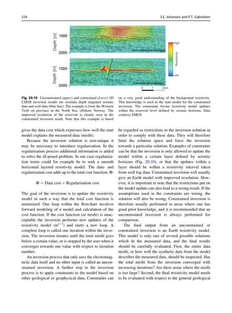
can be that the inversion is only allowed to update the
model within a certain layer defined by seismic
horizons (Fig. 20.10), or that the updates within a
layer should be within a resistivity interval taken
from well log data. Constrained inversion will usually
give an Earth model with improved resolution. However, it is important to note that the restrictions put on
the model update can also lead to a wrong result. If the
assumptions used in the constraints are wrong, the
solution will also be wrong. Constrained inversion is
therefore usually performed in areas where one has
good prior knowledge, and it is recommended that an
unconstrained inversion is always performed for
comparison.
The final output from an unconstrained or
constrained inversion is an Earth resistivity model.
This model is only one of several possible solutions
which fit the measured data, and the final results
should be carefully evaluated. First, the entire data
misfit, or how well the synthetic data from the model
describes the measured data, should be inspected. Has
the total misfit from the inversion converged with
increasing iterations? Are there areas where the misfit
is too large? Second, the final resistivity model needs
to be evaluated with respect to the general geological
Fig. 20.10 Unconstrained (upper) and constrained (lower) 3D
CSEM inversion results are overlain depth migrated seismic
data and well data (blue line). The example is from the Western
Troll oil province in the North Sea, offshore Norway. The
improved resolution of the reservoir is clearly seen in the
constrained inversion result. Note that this example is based
on a very good understanding of the background resistivity.
This knowledge is used in the start model for the constrained
inversion. The constraints favour resistivity model updates
within the reservoir level defined by seismic horizons. Data
courtesy EMGS
524
S.E. Johansen and P.T. Gabrielsen
model explains the measured data (misfit).
Because the inversion solution is non-unique it
may be necessary to introduce regularisation. In the
regularisation process additional information is added
to solve the ill-posed problem. In our case regularization terms could for example be to seek a smooth
horizontal layered resistivity model. The data- and
regularisation cost adds up to the total cost function, Φ:
Φ ¼ Data cost þ Regularisation cost
The goal of the inversion is to update the resistivity
model in such a way that the total cost function is
minimised. One loop within the flowchart involves
forward modeling of a model and calculation of the
cost function. If the cost function (or misfit) is unacceptable the inversion performs new updates of the
resistivity model (m
iþ1 ) and starts a new loop. A
complete loop is called one iteration within the inversion. The inversion iterates until the total misfit goes
below a certain value, or is stopped by the user when it
converges towards one value with respect to iteration
number.
An inversion process that only uses the electromagnetic data itself and no other input is called an unconstrained inversion. A further step in the inversion
process is to apply constraints to the model based on
other geological or geophysical data. Constraints can
be regarded as restrictions to the inversion solution in
order to comply with these data. They will therefore
limit the solution space and force the inversion
towards a particular solution. Examples of constraints
can be that the inversion is only allowed to update the
model within a certain layer defined by seismic
horizons (Fig. 20.10), or that the updates within a
layer should be within a resistivity interval taken
from well log data. Constrained inversion will usually
give an Earth model with improved resolution. However, it is important to note that the restrictions put on
the model update can also lead to a wrong result. If the
assumptions used in the constraints are wrong, the
solution will also be wrong. Constrained inversion is
therefore usually performed in areas where one has
good prior knowledge, and it is recommended that an
unconstrained inversion is always performed for
comparison.
The final output from an unconstrained or
constrained inversion is an Earth resistivity model.
This model is only one of several possible solutions
which fit the measured data, and the final results
should be carefully evaluated. First, the entire data
misfit, or how well the synthetic data from the model
describes the measured data, should be inspected. Has
the total misfit from the inversion converged with
increasing iterations? Are there areas where the misfit
is too large? Second, the final resistivity model needs
to be evaluated with respect to the general geological
Fig. 20.10 Unconstrained (upper) and constrained (lower) 3D
CSEM inversion results are overlain depth migrated seismic
data and well data (blue line). The example is from the Western
Troll oil province in the North Sea, offshore Norway. The
improved resolution of the reservoir is clearly seen in the
constrained inversion result. Note that this example is based
on a very good understanding of the background resistivity.
This knowledge is used in the start model for the constrained
inversion. The constraints favour resistivity model updates
within the reservoir level defined by seismic horizons. Data
courtesy EMGS
524
S.E. Johansen and P.T. Gabrielsen