

resistivity contrast of 40 Ωm, or a target net pay thickness of 40 m and a resistivity contrast of 50 Ωm. These
two scenarios will give approximately equal CSEM
response if the burial depths are comparable. The
transverse resistance is one of the main parameters
that control the CSEM sensitivity.
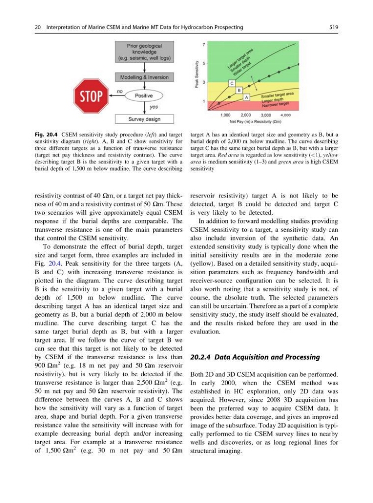
To demonstrate the effect of burial depth, target
size and target form, three examples are included in
Fig. 20.4. Peak sensitivity for the three targets (A,
B and C) with increasing transverse resistance is
plotted in the diagram. The curve describing target
B is the sensitivity to a given target with a burial
depth of 1,500 m below mudline. The curve
describing target A has an identical target size and
geometry as B, but a burial depth of 2,000 m below
mudline. The curve describing target C has the
same target burial depth as B, but with a larger
target area. If we follow the curve of target B we
can see that this target is not likely to be detected
by CSEM if the transverse resistance is less than
900 Ωm
2 (e.g. 18 m net pay and 50 Ωm reservoir
resistivity), but is very likely to be detected if the
transverse resistance is larger than 2,500 Ωm
2 (e.g.
50 m net pay and 50 Ωm reservoir resistivity). The
difference between the curves A, B and C shows
how the sensitivity will vary as a function of target
area, shape and burial depth. For a given transverse
resistance value the sensitivity will increase with for
example decreasing burial depth and/or increasing
target area. For example at a transverse resistance
of 1,500 Ωm
2 (e.g. 30 m net pay and 50 Ωm
reservoir resistivity) target A is not likely to be
detected, target B could be detected and target C
is very likely to be detected.
In addition to forward modelling studies providing
CSEM sensitivity to a target, a sensitivity study can
also include inversion of the synthetic data. An
extended sensitivity study is typically done when the
initial sensitivity results are in the moderate zone
(yellow). Based on a detailed sensitivity study, acquisition parameters such as frequency bandwidth and
receiver-source configuration can be selected. It is
also worth noting that a sensitivity study is not, of
course, the absolute truth. The selected parameters
can still be uncertain. Therefore as a part of a complete
sensitivity study, the study itself should be evaluated,
and the results risked before they are used in the
evaluation.
20.2.4 Data Acquisition and Processing
Both 2D and 3D CSEM acquisition can be performed.
In early 2000, when the CSEM method was
established in HC exploration, only 2D data was
acquired. However, since 2008 3D acquisition has
been the preferred way to acquire CSEM data. It
provides better data coverage, and gives an improved
image of the subsurface. Today 2D acquisition is typically performed to tie CSEM survey lines to nearby
wells and discoveries, or as long regional lines for
structural imaging.
Fig. 20.4 CSEM sensitivity study procedure (left) and target
sensitivity diagram (right). A, B and C show sensitivity for
three different targets as a function of transverse resistance
(target net pay thickness and resistivity contrast). The curve
describing target B is the sensitivity to a given target with a
burial depth of 1,500 m below mudline. The curve describing
target A has an identical target size and geometry as B, but a
burial depth of 2,000 m below mudline. The curve describing
target C has the same target burial depth as B, but with a larger
target area. Red area is regarded as low sensitivity (<1), yellow
area is medium sensitivity (1–3) and green area is high CSEM
sensitivity
20 Interpretation of Marine CSEM and Marine MT Data for Hydrocarbon Prospecting
519
two scenarios will give approximately equal CSEM
response if the burial depths are comparable. The
transverse resistance is one of the main parameters
that control the CSEM sensitivity.
To demonstrate the effect of burial depth, target
size and target form, three examples are included in
Fig. 20.4. Peak sensitivity for the three targets (A,
B and C) with increasing transverse resistance is
plotted in the diagram. The curve describing target
B is the sensitivity to a given target with a burial
depth of 1,500 m below mudline. The curve
describing target A has an identical target size and
geometry as B, but a burial depth of 2,000 m below
mudline. The curve describing target C has the
same target burial depth as B, but with a larger
target area. If we follow the curve of target B we
can see that this target is not likely to be detected
by CSEM if the transverse resistance is less than
900 Ωm
2 (e.g. 18 m net pay and 50 Ωm reservoir
resistivity), but is very likely to be detected if the
transverse resistance is larger than 2,500 Ωm
2 (e.g.
50 m net pay and 50 Ωm reservoir resistivity). The
difference between the curves A, B and C shows
how the sensitivity will vary as a function of target
area, shape and burial depth. For a given transverse
resistance value the sensitivity will increase with for
example decreasing burial depth and/or increasing
target area. For example at a transverse resistance
of 1,500 Ωm
2 (e.g. 30 m net pay and 50 Ωm
reservoir resistivity) target A is not likely to be
detected, target B could be detected and target C
is very likely to be detected.
In addition to forward modelling studies providing
CSEM sensitivity to a target, a sensitivity study can
also include inversion of the synthetic data. An
extended sensitivity study is typically done when the
initial sensitivity results are in the moderate zone
(yellow). Based on a detailed sensitivity study, acquisition parameters such as frequency bandwidth and
receiver-source configuration can be selected. It is
also worth noting that a sensitivity study is not, of
course, the absolute truth. The selected parameters
can still be uncertain. Therefore as a part of a complete
sensitivity study, the study itself should be evaluated,
and the results risked before they are used in the
evaluation.
20.2.4 Data Acquisition and Processing
Both 2D and 3D CSEM acquisition can be performed.
In early 2000, when the CSEM method was
established in HC exploration, only 2D data was
acquired. However, since 2008 3D acquisition has
been the preferred way to acquire CSEM data. It
provides better data coverage, and gives an improved
image of the subsurface. Today 2D acquisition is typically performed to tie CSEM survey lines to nearby
wells and discoveries, or as long regional lines for
structural imaging.
Fig. 20.4 CSEM sensitivity study procedure (left) and target
sensitivity diagram (right). A, B and C show sensitivity for
three different targets as a function of transverse resistance
(target net pay thickness and resistivity contrast). The curve
describing target B is the sensitivity to a given target with a
burial depth of 1,500 m below mudline. The curve describing
target A has an identical target size and geometry as B, but a
burial depth of 2,000 m below mudline. The curve describing
target C has the same target burial depth as B, but with a larger
target area. Red area is regarded as low sensitivity (<1), yellow
area is medium sensitivity (1–3) and green area is high CSEM
sensitivity
20 Interpretation of Marine CSEM and Marine MT Data for Hydrocarbon Prospecting
519