

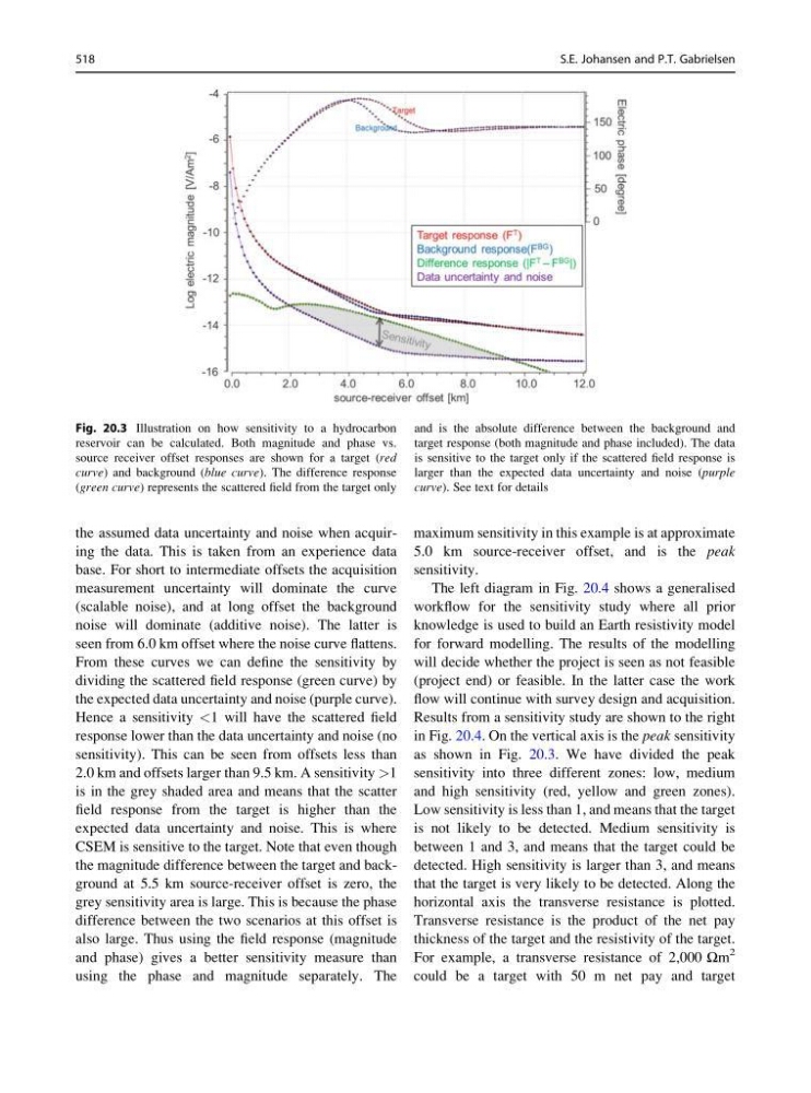
the assumed data uncertainty and noise when acquiring the data. This is taken from an experience data
base. For short to intermediate offsets the acquisition
measurement uncertainty will dominate the curve
(scalable noise), and at long offset the background
noise will dominate (additive noise). The latter is
seen from 6.0 km offset where the noise curve flattens.
From these curves we can define the sensitivity by
dividing the scattered field response (green curve) by
the expected data uncertainty and noise (purple curve).
Hence a sensitivity <1 will have the scattered field
response lower than the data uncertainty and noise (no
sensitivity). This can be seen from offsets less than
2.0 km and offsets larger than 9.5 km. A sensitivity >1
is in the grey shaded area and means that the scatter
field response from the target is higher than the
expected data uncertainty and noise. This is where
CSEM is sensitive to the target. Note that even though
the magnitude difference between the target and background at 5.5 km source-receiver offset is zero, the
grey sensitivity area is large. This is because the phase
difference between the two scenarios at this offset is
also large. Thus using the field response (magnitude
and phase) gives a better sensitivity measure than
using the phase and magnitude separately. The
maximum sensitivity in this example is at approximate
5.0 km source-receiver offset, and is the peak
sensitivity.
The left diagram in Fig. 20.4 shows a generalised
workflow for the sensitivity study where all prior
knowledge is used to build an Earth resistivity model
for forward modelling. The results of the modelling
will decide whether the project is seen as not feasible
(project end) or feasible. In the latter case the work
flow will continue with survey design and acquisition.
Results from a sensitivity study are shown to the right
in Fig. 20.4. On the vertical axis is the peak sensitivity
as shown in Fig. 20.3. We have divided the peak
sensitivity into three different zones: low, medium
and high sensitivity (red, yellow and green zones).
Low sensitivity is less than 1, and means that the target
is not likely to be detected. Medium sensitivity is
between 1 and 3, and means that the target could be
detected. High sensitivity is larger than 3, and means
that the target is very likely to be detected. Along the
horizontal axis the transverse resistance is plotted.
Transverse resistance is the product of the net pay
thickness of the target and the resistivity of the target.
For example, a transverse resistance of 2,000 Ωm
2
could be a target with 50 m net pay and target
Fig. 20.3 Illustration on how sensitivity to a hydrocarbon
reservoir can be calculated. Both magnitude and phase vs.
source receiver offset responses are shown for a target (red
curve) and background (blue curve). The difference response
(green curve) represents the scattered field from the target only
and is the absolute difference between the background and
target response (both magnitude and phase included). The data
is sensitive to the target only if the scattered field response is
larger than the expected data uncertainty and noise (purple
curve). See text for details
518
S.E. Johansen and P.T. Gabrielsen
base. For short to intermediate offsets the acquisition
measurement uncertainty will dominate the curve
(scalable noise), and at long offset the background
noise will dominate (additive noise). The latter is
seen from 6.0 km offset where the noise curve flattens.
From these curves we can define the sensitivity by
dividing the scattered field response (green curve) by
the expected data uncertainty and noise (purple curve).
Hence a sensitivity <1 will have the scattered field
response lower than the data uncertainty and noise (no
sensitivity). This can be seen from offsets less than
2.0 km and offsets larger than 9.5 km. A sensitivity >1
is in the grey shaded area and means that the scatter
field response from the target is higher than the
expected data uncertainty and noise. This is where
CSEM is sensitive to the target. Note that even though
the magnitude difference between the target and background at 5.5 km source-receiver offset is zero, the
grey sensitivity area is large. This is because the phase
difference between the two scenarios at this offset is
also large. Thus using the field response (magnitude
and phase) gives a better sensitivity measure than
using the phase and magnitude separately. The
maximum sensitivity in this example is at approximate
5.0 km source-receiver offset, and is the peak
sensitivity.
The left diagram in Fig. 20.4 shows a generalised
workflow for the sensitivity study where all prior
knowledge is used to build an Earth resistivity model
for forward modelling. The results of the modelling
will decide whether the project is seen as not feasible
(project end) or feasible. In the latter case the work
flow will continue with survey design and acquisition.
Results from a sensitivity study are shown to the right
in Fig. 20.4. On the vertical axis is the peak sensitivity
as shown in Fig. 20.3. We have divided the peak
sensitivity into three different zones: low, medium
and high sensitivity (red, yellow and green zones).
Low sensitivity is less than 1, and means that the target
is not likely to be detected. Medium sensitivity is
between 1 and 3, and means that the target could be
detected. High sensitivity is larger than 3, and means
that the target is very likely to be detected. Along the
horizontal axis the transverse resistance is plotted.
Transverse resistance is the product of the net pay
thickness of the target and the resistivity of the target.
For example, a transverse resistance of 2,000 Ωm
2
could be a target with 50 m net pay and target
Fig. 20.3 Illustration on how sensitivity to a hydrocarbon
reservoir can be calculated. Both magnitude and phase vs.
source receiver offset responses are shown for a target (red
curve) and background (blue curve). The difference response
(green curve) represents the scattered field from the target only
and is the absolute difference between the background and
target response (both magnitude and phase included). The data
is sensitive to the target only if the scattered field response is
larger than the expected data uncertainty and noise (purple
curve). See text for details
518
S.E. Johansen and P.T. Gabrielsen