

of travel time and amplitude changes. We notice that
the differences at zero offset are negligible, as
expected.
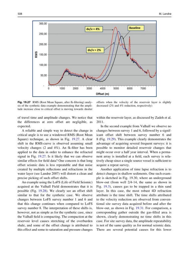
A reliable and simple way to detect the change in
critical angle is to use a windowed RMS (Root Mean
Square) technique, as shown in Fig. 19.27. A clear
shift in the RMS-curve is observed assuming small
velocity changes (2 and 4%). An fk-filter has been
applied to the data in order to enhance the refracted
signal in Fig. 19.27. Is it likely that we can observe
similar effects for field data? One concern is that long
offset seismic data is less repeatable and that noise
created by multiple reflections and refractions in the
water layer (see Landrø 2007) will distort a clean and
precise picking of such offset shifts.
An example using the LoFS (Life of Field Seismic)
acquired at the Valhall Field demonstrates that it is
possible (Fig. 19.28). We clearly see an offset shift
similar to that for the synthetic case. We observe
changes between LoFS survey number 1 and 6 and
that this change continues when compared to LoFS
survey number 8. The interpretation of these shifts is,
however, not as simple as for the synthetic case, since
the Valhall field is compacting. The compaction at the
reservoir level causes stretching of the overburden
shale, and some of the offset change is attributed to
this effect and some to saturation and pressure changes
within the reservoir layer, as discussed by Zadeh et al.
2011.
In the second example from Valhall we observe no
changes between survey 1 and 6, followed by a significant offset shift between survey number 6 and
8 (Fig. 19.29). This example clearly demonstrates the
advantage of acquiring several frequent surveys: it is
possible to monitor detailed reservoir changes that
might occur over a half year interval. When a permanent array is installed at a field, each survey is relatively cheap since a single source vessel is sufficient to
acquire a repeat survey.
Another application of time lapse refraction is to
detect changes in shallow sediments. One such example is sketched in Fig. 19.30, where an underground
blow-out (from well 2/4-14, the same as shown in
Fig. 19.3), causes gas to be trapped in a thin sand
layer. In this case, the most robust 4D refraction
attribute is the time shift. The time shifts attributed
to the velocity reduction are observed from conventional site survey data acquired before and after the
blow-out, as shown in Fig. 19.31. For comparison, a
corresponding gather outside the gas-filled area is
shown, clearly demonstrating no time shifts in this
case. For site survey data, the amplitude repeatability
is not of the same quality as for normal seismic data.
There are several potential causes for this lower
Fig. 19.27 RMS (Root Mean Square, after fk-filtering) analysis of the synthetic data example demonstrating that the amplitude increase close to critical offset is moving towards shorter
offsets when the velocity of the reservoir layer is slightly
decreased (2% and 4% reduction, respectively)
508
M. Landrø
the differences at zero offset are negligible, as
expected.
A reliable and simple way to detect the change in
critical angle is to use a windowed RMS (Root Mean
Square) technique, as shown in Fig. 19.27. A clear
shift in the RMS-curve is observed assuming small
velocity changes (2 and 4%). An fk-filter has been
applied to the data in order to enhance the refracted
signal in Fig. 19.27. Is it likely that we can observe
similar effects for field data? One concern is that long
offset seismic data is less repeatable and that noise
created by multiple reflections and refractions in the
water layer (see Landrø 2007) will distort a clean and
precise picking of such offset shifts.
An example using the LoFS (Life of Field Seismic)
acquired at the Valhall Field demonstrates that it is
possible (Fig. 19.28). We clearly see an offset shift
similar to that for the synthetic case. We observe
changes between LoFS survey number 1 and 6 and
that this change continues when compared to LoFS
survey number 8. The interpretation of these shifts is,
however, not as simple as for the synthetic case, since
the Valhall field is compacting. The compaction at the
reservoir level causes stretching of the overburden
shale, and some of the offset change is attributed to
this effect and some to saturation and pressure changes
within the reservoir layer, as discussed by Zadeh et al.
2011.
In the second example from Valhall we observe no
changes between survey 1 and 6, followed by a significant offset shift between survey number 6 and
8 (Fig. 19.29). This example clearly demonstrates the
advantage of acquiring several frequent surveys: it is
possible to monitor detailed reservoir changes that
might occur over a half year interval. When a permanent array is installed at a field, each survey is relatively cheap since a single source vessel is sufficient to
acquire a repeat survey.
Another application of time lapse refraction is to
detect changes in shallow sediments. One such example is sketched in Fig. 19.30, where an underground
blow-out (from well 2/4-14, the same as shown in
Fig. 19.3), causes gas to be trapped in a thin sand
layer. In this case, the most robust 4D refraction
attribute is the time shift. The time shifts attributed
to the velocity reduction are observed from conventional site survey data acquired before and after the
blow-out, as shown in Fig. 19.31. For comparison, a
corresponding gather outside the gas-filled area is
shown, clearly demonstrating no time shifts in this
case. For site survey data, the amplitude repeatability
is not of the same quality as for normal seismic data.
There are several potential causes for this lower
Fig. 19.27 RMS (Root Mean Square, after fk-filtering) analysis of the synthetic data example demonstrating that the amplitude increase close to critical offset is moving towards shorter
offsets when the velocity of the reservoir layer is slightly
decreased (2% and 4% reduction, respectively)
508
M. Landrø