

developed methods to estimate the thickness of CO 2
layers, which makes it possible to estimate volumes.
Another key parameter is CO 2 saturation, which can
be estimated using rock physics measurements and
models. Although the precision in both 4D seismic
methods and rock physics is increasing, there is no
doubt that precise estimates are hard to achieve, and
therefore we need to improve existing methods and
learn how to combine several methods in order to
decrease the uncertainties associated with these monitoring methods.
19.11 Time-lapse Refraction Methods
Refraction methods are among the oldest methods in
seismic exploration. The term refraction is not unique
or precise. According to Sheriff (2002) it has two
meanings, first to change direction (following Snell’s
law) and second to involve head waves. In this chapter
I will use a relaxed interpretation which means that the
term includes head waves, diving waves and
reflections close to critical angle. Maybe long offset
time-lapse seismic is more correct. Within petroleum
geophysics, one of the first proposals to exploit this
type of data for 4D purposes was presented by Landrø
et al. 2004. It was suggested that 4D refraction analysis could be of potential benefit for carbonate
reservoirs. The basic condition for generation of head
waves is that the incidence angle of a seismic wave is
larger than the critical angle θ C :
sin θ C ¼
v 1
v 2
(19.16)
where v 1 and v 2 denote the velocity above and below
the top reservoir (or the target) interface. It is evident
from this equation that there has to be a velocity
increase in order to create head waves for incidence
angles greater than the critical angle. This is also one
of the major limitations for this method: it does not
work for interfaces where the velocity contrast is weak
or decreasing. Another weakness of the method is that
it relies on dominantly horizontal wave propagation,
and therefore it is most robust for detecting velocity
changes that are laterally extensive. Small, localised
4D anomalies are better resolved by using conventional 4D reflection methods. However, in a situation
where the velocity changes caused by production are
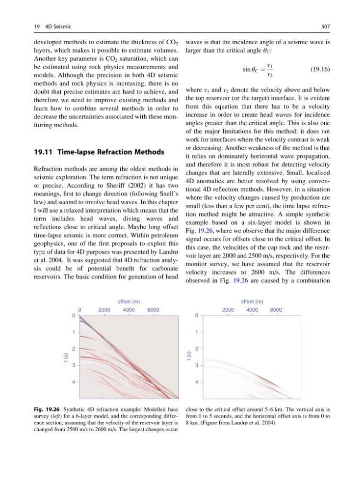
small (less than a few per cent), the time lapse refraction method might be attractive. A simple synthetic
example based on a six-layer model is shown in
Fig. 19.26, where we observe that the major difference
signal occurs for offsets close to the critical offset. In
this case, the velocities of the cap rock and the reservoir layer are 2000 and 2500 m/s, respectively. For the
monitor survey, we have assumed that the reservoir
velocity increases to 2600 m/s. The differences
observed in Fig. 19.26 are caused by a combination
0
0
1
2
3
4
t (s)
2000
4000
6000
offset (m)
0
1
2
3
4
t (s)
2000
4000
6000
offset (m)
Fig. 19.26 Synthetic 4D refraction example: Modelled base
survey (left) for a 6-layer model, and the corresponding difference section, assuming that the velocity of the reservoir layer is
changed from 2500 m/s to 2600 m/s. The largest changes occur
close to the critical offset around 5–6 km. The vertical axis is
from 0 to 5 seconds, and the horizontal offset axis is from 0 to
8 km. (Figure from Landrø et al. 2004)
19 4D Seismic
507
layers, which makes it possible to estimate volumes.
Another key parameter is CO 2 saturation, which can
be estimated using rock physics measurements and
models. Although the precision in both 4D seismic
methods and rock physics is increasing, there is no
doubt that precise estimates are hard to achieve, and
therefore we need to improve existing methods and
learn how to combine several methods in order to
decrease the uncertainties associated with these monitoring methods.
19.11 Time-lapse Refraction Methods
Refraction methods are among the oldest methods in
seismic exploration. The term refraction is not unique
or precise. According to Sheriff (2002) it has two
meanings, first to change direction (following Snell’s
law) and second to involve head waves. In this chapter
I will use a relaxed interpretation which means that the
term includes head waves, diving waves and
reflections close to critical angle. Maybe long offset
time-lapse seismic is more correct. Within petroleum
geophysics, one of the first proposals to exploit this
type of data for 4D purposes was presented by Landrø
et al. 2004. It was suggested that 4D refraction analysis could be of potential benefit for carbonate
reservoirs. The basic condition for generation of head
waves is that the incidence angle of a seismic wave is
larger than the critical angle θ C :
sin θ C ¼
v 1
v 2
(19.16)
where v 1 and v 2 denote the velocity above and below
the top reservoir (or the target) interface. It is evident
from this equation that there has to be a velocity
increase in order to create head waves for incidence
angles greater than the critical angle. This is also one
of the major limitations for this method: it does not
work for interfaces where the velocity contrast is weak
or decreasing. Another weakness of the method is that
it relies on dominantly horizontal wave propagation,
and therefore it is most robust for detecting velocity
changes that are laterally extensive. Small, localised
4D anomalies are better resolved by using conventional 4D reflection methods. However, in a situation
where the velocity changes caused by production are
small (less than a few per cent), the time lapse refraction method might be attractive. A simple synthetic
example based on a six-layer model is shown in
Fig. 19.26, where we observe that the major difference
signal occurs for offsets close to the critical offset. In
this case, the velocities of the cap rock and the reservoir layer are 2000 and 2500 m/s, respectively. For the
monitor survey, we have assumed that the reservoir
velocity increases to 2600 m/s. The differences
observed in Fig. 19.26 are caused by a combination
0
0
1
2
3
4
t (s)
2000
4000
6000
offset (m)
0
1
2
3
4
t (s)
2000
4000
6000
offset (m)
Fig. 19.26 Synthetic 4D refraction example: Modelled base
survey (left) for a 6-layer model, and the corresponding difference section, assuming that the velocity of the reservoir layer is
changed from 2500 m/s to 2600 m/s. The largest changes occur
close to the critical offset around 5–6 km. The vertical axis is
from 0 to 5 seconds, and the horizontal offset axis is from 0 to
8 km. (Figure from Landrø et al. 2004)
19 4D Seismic
507