

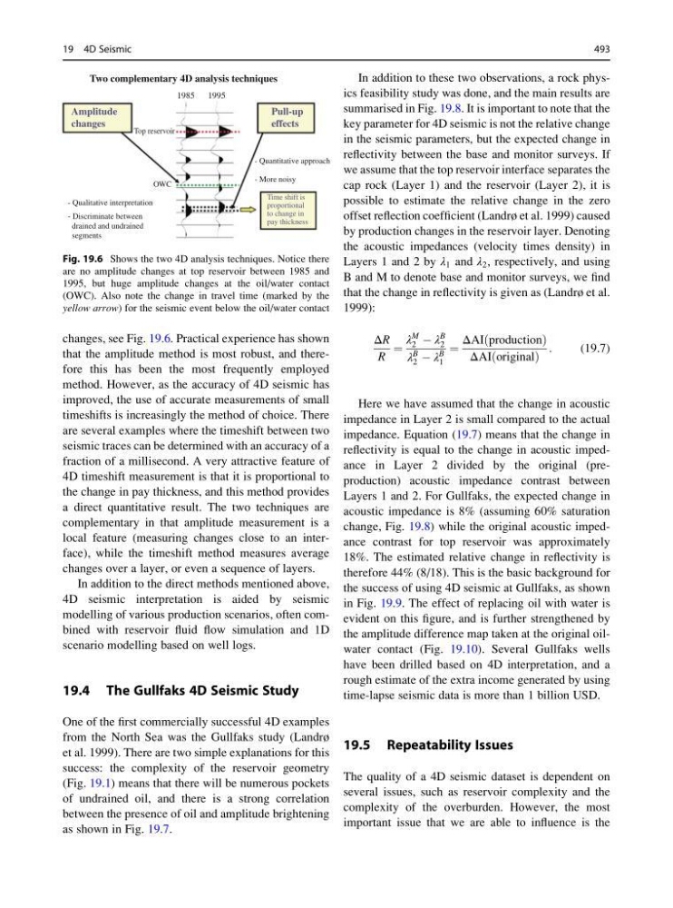
changes, see Fig. 19.6. Practical experience has shown
that the amplitude method is most robust, and therefore this has been the most frequently employed
method. However, as the accuracy of 4D seismic has
improved, the use of accurate measurements of small
timeshifts is increasingly the method of choice. There
are several examples where the timeshift between two
seismic traces can be determined with an accuracy of a
fraction of a millisecond. A very attractive feature of
4D timeshift measurement is that it is proportional to
the change in pay thickness, and this method provides
a direct quantitative result. The two techniques are
complementary in that amplitude measurement is a
local feature (measuring changes close to an interface), while the timeshift method measures average
changes over a layer, or even a sequence of layers.
In addition to the direct methods mentioned above,
4D seismic interpretation is aided by seismic
modelling of various production scenarios, often combined with reservoir fluid flow simulation and 1D
scenario modelling based on well logs.
19.4 The Gullfaks 4D Seismic Study
One of the first commercially successful 4D examples
from the North Sea was the Gullfaks study (Landrø
et al. 1999). There are two simple explanations for this
success: the complexity of the reservoir geometry
(Fig. 19.1) means that there will be numerous pockets
of undrained oil, and there is a strong correlation
between the presence of oil and amplitude brightening
as shown in Fig. 19.7.
In addition to these two observations, a rock physics feasibility study was done, and the main results are
summarised in Fig. 19.8. It is important to note that the
key parameter for 4D seismic is not the relative change
in the seismic parameters, but the expected change in
reflectivity between the base and monitor surveys. If
we assume that the top reservoir interface separates the
cap rock (Layer 1) and the reservoir (Layer 2), it is
possible to estimate the relative change in the zero
offset reflection coefficient (Landrø et al. 1999) caused
by production changes in the reservoir layer. Denoting
the acoustic impedances (velocity times density) in
Layers 1 and 2 by λ 1 and λ 2 , respectively, and using
B and M to denote base and monitor surveys, we find
that the change in reflectivity is given as (Landrø et al.
1999):
ΔR
R
¼
λ
M
2 À λ
B
2
λ
B
2 À λ
B
1
¼
ΔAIðproductionÞ
ΔAIðoriginalÞ
:
(19.7)
Here we have assumed that the change in acoustic
impedance in Layer 2 is small compared to the actual
impedance. Equation (19.7) means that the change in
reflectivity is equal to the change in acoustic impedance in Layer 2 divided by the original (preproduction) acoustic impedance contrast between
Layers 1 and 2. For Gullfaks, the expected change in
acoustic impedance is 8% (assuming 60% saturation
change, Fig. 19.8) while the original acoustic impedance contrast for top reservoir was approximately
18%. The estimated relative change in reflectivity is
therefore 44% (8/18). This is the basic background for
the success of using 4D seismic at Gullfaks, as shown
in Fig. 19.9. The effect of replacing oil with water is
evident on this figure, and is further strengthened by
the amplitude difference map taken at the original oilwater contact (Fig. 19.10). Several Gullfaks wells
have been drilled based on 4D interpretation, and a
rough estimate of the extra income generated by using
time-lapse seismic data is more than 1 billion USD.
19.5 Repeatability Issues
The quality of a 4D seismic dataset is dependent on
several issues, such as reservoir complexity and the
complexity of the overburden. However, the most
important issue that we are able to influence is the
Two complementary 4D analysis techniques
- Qualitative interpretation
- More noisy
- Quantitative approach
Top reservoir
1985 1995
OWC
- Discriminate between
drained and undrained
segments
Amplitude
changes
Pull-up
effects
Time shift is
proportional
to change in
pay thickness
Fig. 19.6 Shows the two 4D analysis techniques. Notice there
are no amplitude changes at top reservoir between 1985 and
1995, but huge amplitude changes at the oil/water contact
(OWC). Also note the change in travel time (marked by the
yellow arrow) for the seismic event below the oil/water contact
19 4D Seismic
493
that the amplitude method is most robust, and therefore this has been the most frequently employed
method. However, as the accuracy of 4D seismic has
improved, the use of accurate measurements of small
timeshifts is increasingly the method of choice. There
are several examples where the timeshift between two
seismic traces can be determined with an accuracy of a
fraction of a millisecond. A very attractive feature of
4D timeshift measurement is that it is proportional to
the change in pay thickness, and this method provides
a direct quantitative result. The two techniques are
complementary in that amplitude measurement is a
local feature (measuring changes close to an interface), while the timeshift method measures average
changes over a layer, or even a sequence of layers.
In addition to the direct methods mentioned above,
4D seismic interpretation is aided by seismic
modelling of various production scenarios, often combined with reservoir fluid flow simulation and 1D
scenario modelling based on well logs.
19.4 The Gullfaks 4D Seismic Study
One of the first commercially successful 4D examples
from the North Sea was the Gullfaks study (Landrø
et al. 1999). There are two simple explanations for this
success: the complexity of the reservoir geometry
(Fig. 19.1) means that there will be numerous pockets
of undrained oil, and there is a strong correlation
between the presence of oil and amplitude brightening
as shown in Fig. 19.7.
In addition to these two observations, a rock physics feasibility study was done, and the main results are
summarised in Fig. 19.8. It is important to note that the
key parameter for 4D seismic is not the relative change
in the seismic parameters, but the expected change in
reflectivity between the base and monitor surveys. If
we assume that the top reservoir interface separates the
cap rock (Layer 1) and the reservoir (Layer 2), it is
possible to estimate the relative change in the zero
offset reflection coefficient (Landrø et al. 1999) caused
by production changes in the reservoir layer. Denoting
the acoustic impedances (velocity times density) in
Layers 1 and 2 by λ 1 and λ 2 , respectively, and using
B and M to denote base and monitor surveys, we find
that the change in reflectivity is given as (Landrø et al.
1999):
ΔR
R
¼
λ
M
2 À λ
B
2
λ
B
2 À λ
B
1
¼
ΔAIðproductionÞ
ΔAIðoriginalÞ
:
(19.7)
Here we have assumed that the change in acoustic
impedance in Layer 2 is small compared to the actual
impedance. Equation (19.7) means that the change in
reflectivity is equal to the change in acoustic impedance in Layer 2 divided by the original (preproduction) acoustic impedance contrast between
Layers 1 and 2. For Gullfaks, the expected change in
acoustic impedance is 8% (assuming 60% saturation
change, Fig. 19.8) while the original acoustic impedance contrast for top reservoir was approximately
18%. The estimated relative change in reflectivity is
therefore 44% (8/18). This is the basic background for
the success of using 4D seismic at Gullfaks, as shown
in Fig. 19.9. The effect of replacing oil with water is
evident on this figure, and is further strengthened by
the amplitude difference map taken at the original oilwater contact (Fig. 19.10). Several Gullfaks wells
have been drilled based on 4D interpretation, and a
rough estimate of the extra income generated by using
time-lapse seismic data is more than 1 billion USD.
19.5 Repeatability Issues
The quality of a 4D seismic dataset is dependent on
several issues, such as reservoir complexity and the
complexity of the overburden. However, the most
important issue that we are able to influence is the
Two complementary 4D analysis techniques
- Qualitative interpretation
- More noisy
- Quantitative approach
Top reservoir
1985 1995
OWC
- Discriminate between
drained and undrained
segments
Amplitude
changes
Pull-up
effects
Time shift is
proportional
to change in
pay thickness
Fig. 19.6 Shows the two 4D analysis techniques. Notice there
are no amplitude changes at top reservoir between 1985 and
1995, but huge amplitude changes at the oil/water contact
(OWC). Also note the change in travel time (marked by the
yellow arrow) for the seismic event below the oil/water contact
19 4D Seismic
493