

In addition, various contact models have been proposed to estimate the effective modulus of a rock.
Mavko, Mukerji and Dvorkin present some of these
models in their rock physics handbook (1998). The
Hertz-Mindlin model (Mindlin 1949) can be used to
describe the properties of pre-compacted granular
rocks. The effective bulk modulus of dry random
identical sphere packing is given by:
K eff ¼
C
2
p ð1 À φ
2
ÞG
2 P
18π 2 ð1 À σÞ
2
(
) 1
3
(19.1)
where C p is the number of contact points per grain, φ is
porosity, G is the shear modulus of the solid grains, σ
is the Poisson ratio of the solid grains and P is the
effective pressure (that is P ¼ P eff ). The shear modulus is given as:
G eff ¼
3C
2
p ð1 À φÞ
2 G
2 P
2π 2 ð1 À σÞ
2
(
) 1
3 5 À 4σ
5ð2 À σÞ
(19.2)
This leads to:
V P ¼
ffiffiffiffiffiffiffiffiffiffiffiffiffiffiffiffiffiffiffiffiffiffiffi ffi
K eff þ
4
3 G eff
ρ
s
(19.3)
V S ¼
ffiffiffiffiffiffiffiffi
G eff
ρ
s
(19.4)
where V p and V s are P- and S-wave velocities, respectively, and ρ is the sandstone density. Inserting
Eqs. (19.1) and (19.2) into Eqs. (19.3) and (19.4) and
computing the V p =V s ratio, yields (assuming σ ¼ 0):
V P
V S
¼
ffiffi ffi
2
p :
(19.5)
This means that according to the simplest granular
model (Hertz-Mindlin), the V p =V s ratio should be constant as a function of confining pressure if we assume
the rock is dry. The Hertz-Mindlin model assumes the
sand grains are spherical and that there is a certain area
of grain-to-grain contacts. A major shortcoming of the
model is that at the limit of unconsolidated sands, both
the P- and S-wave velocities will have the same
behaviour with respect to pressure changes, as shown
in Eq. (19.5). Combining with the Gassmann (1951)
model (i.e. introducing fluids in the pore system of the
rock), will ensure that the P-wave velocity approaches
the fluid velocity for zero effective stress, and not zero
as in the Hertz-Mindlin model (dry rock assumption).
If we assume that the in situ (base survey) effective
pressure is P 0 we see from Eq. (19.3) that the relative
P-wave velocity versus effective pressure is given as:
V P
V P 0
¼
P
P 0
1
6
(19.6)
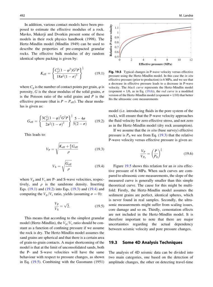
Figure 19.5 shows this relation for an in situ effective pressure of 6 MPa. When such curves are compared to ultrasonic core measurements, the slope of the
measured curve is generally smaller than this simple
theoretical curve. The cause for this might be multifold: Firstly, the Hertz-Mindlin model assumes the
sediment grains are perfect, identical spheres, which
is never found in real samples. Secondly, the ultrasonic measurements might suffer from scaling issues,
core damage and so on. Thirdly, cementation effects
are not included in the Hertz-Mindlin model. It is
therefore important to note that there are major
uncertainties regarding the actual dependency
between seismic velocity and pore pressure changes.
19.3 Some 4D Analysis Techniques
The analysis of 4D seismic data can be divided into
two main categories, one based on the detection of
amplitude changes, the other on detecting travel-time
1.1
1
0.9
Relative P-wave velocity
0.8
0.7
0.6
0.5
0
2
4
6
Effective pressure (MPa)
8
1 0
1 2
Fig. 19.5 Typical changes in P-wave velocity versus effective
pressure using the Hertz-Mindlin model. In this case the in situ
effective pressure (prior to production) is 6 MPa, and we see that
a decrease in effective pressure leads to a decrease in P-wave
velocity. The black curve represents the Hertz-Mindlin model
(exponent = 1/6, as in Eq. (19.6)), the red curve is a modified
version of the Hertz-Mindlin model (exponent = 1/10) that better
fits the ultrasonic core measurements
492
M. Landrø
Mavko, Mukerji and Dvorkin present some of these
models in their rock physics handbook (1998). The
Hertz-Mindlin model (Mindlin 1949) can be used to
describe the properties of pre-compacted granular
rocks. The effective bulk modulus of dry random
identical sphere packing is given by:
K eff ¼
C
2
p ð1 À φ
2
ÞG
2 P
18π 2 ð1 À σÞ
2
(
) 1
3
(19.1)
where C p is the number of contact points per grain, φ is
porosity, G is the shear modulus of the solid grains, σ
is the Poisson ratio of the solid grains and P is the
effective pressure (that is P ¼ P eff ). The shear modulus is given as:
G eff ¼
3C
2
p ð1 À φÞ
2 G
2 P
2π 2 ð1 À σÞ
2
(
) 1
3 5 À 4σ
5ð2 À σÞ
(19.2)
This leads to:
V P ¼
ffiffiffiffiffiffiffiffiffiffiffiffiffiffiffiffiffiffiffiffiffiffiffi ffi
K eff þ
4
3 G eff
ρ
s
(19.3)
V S ¼
ffiffiffiffiffiffiffiffi
G eff
ρ
s
(19.4)
where V p and V s are P- and S-wave velocities, respectively, and ρ is the sandstone density. Inserting
Eqs. (19.1) and (19.2) into Eqs. (19.3) and (19.4) and
computing the V p =V s ratio, yields (assuming σ ¼ 0):
V P
V S
¼
ffiffi ffi
2
p :
(19.5)
This means that according to the simplest granular
model (Hertz-Mindlin), the V p =V s ratio should be constant as a function of confining pressure if we assume
the rock is dry. The Hertz-Mindlin model assumes the
sand grains are spherical and that there is a certain area
of grain-to-grain contacts. A major shortcoming of the
model is that at the limit of unconsolidated sands, both
the P- and S-wave velocities will have the same
behaviour with respect to pressure changes, as shown
in Eq. (19.5). Combining with the Gassmann (1951)
model (i.e. introducing fluids in the pore system of the
rock), will ensure that the P-wave velocity approaches
the fluid velocity for zero effective stress, and not zero
as in the Hertz-Mindlin model (dry rock assumption).
If we assume that the in situ (base survey) effective
pressure is P 0 we see from Eq. (19.3) that the relative
P-wave velocity versus effective pressure is given as:
V P
V P 0
¼
P
P 0
1
6
(19.6)
Figure 19.5 shows this relation for an in situ effective pressure of 6 MPa. When such curves are compared to ultrasonic core measurements, the slope of the
measured curve is generally smaller than this simple
theoretical curve. The cause for this might be multifold: Firstly, the Hertz-Mindlin model assumes the
sediment grains are perfect, identical spheres, which
is never found in real samples. Secondly, the ultrasonic measurements might suffer from scaling issues,
core damage and so on. Thirdly, cementation effects
are not included in the Hertz-Mindlin model. It is
therefore important to note that there are major
uncertainties regarding the actual dependency
between seismic velocity and pore pressure changes.
19.3 Some 4D Analysis Techniques
The analysis of 4D seismic data can be divided into
two main categories, one based on the detection of
amplitude changes, the other on detecting travel-time
1.1
1
0.9
Relative P-wave velocity
0.8
0.7
0.6
0.5
0
2
4
6
Effective pressure (MPa)
8
1 0
1 2
Fig. 19.5 Typical changes in P-wave velocity versus effective
pressure using the Hertz-Mindlin model. In this case the in situ
effective pressure (prior to production) is 6 MPa, and we see that
a decrease in effective pressure leads to a decrease in P-wave
velocity. The black curve represents the Hertz-Mindlin model
(exponent = 1/6, as in Eq. (19.6)), the red curve is a modified
version of the Hertz-Mindlin model (exponent = 1/10) that better
fits the ultrasonic core measurements
492
M. Landrø