

over the major northern part of the field, and the initial
interpretation performed shortly after this monitor survey demonstrated a promising potential.
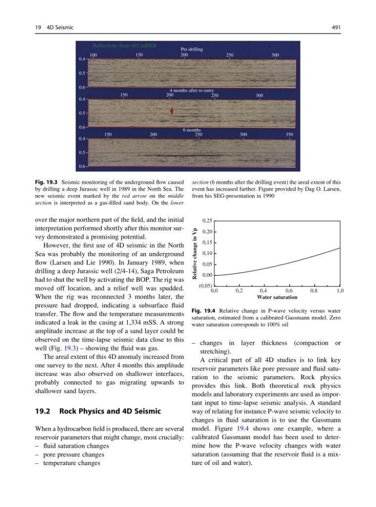
However, the first use of 4D seismic in the North
Sea was probably the monitoring of an underground
flow (Larsen and Lie 1990). In January 1989, when
drilling a deep Jurassic well (2/4-14), Saga Petroleum
had to shut the well by activating the BOP. The rig was
moved off location, and a relief well was spudded.
When the rig was reconnected 3 months later, the
pressure had dropped, indicating a subsurface fluid
transfer. The flow and the temperature measurements
indicated a leak in the casing at 1,334 mSS. A strong
amplitude increase at the top of a sand layer could be
observed on the time-lapse seismic data close to this
well (Fig. 19.3) – showing the fluid was gas.
The areal extent of this 4D anomaly increased from
one survey to the next. After 4 months this amplitude
increase was also observed on shallower interfaces,
probably connected to gas migrating upwards to
shallower sand layers.
19.2 Rock Physics and 4D Seismic
When a hydrocarbon field is produced, there are several
reservoir parameters that might change, most crucially:
– fluid saturation changes
– pore pressure changes
– temperature changes
– changes in layer thickness (compaction or
stretching).
A critical part of all 4D studies is to link key
reservoir parameters like pore pressure and fluid saturation to the seismic parameters. Rock physics
provides this link. Both theoretical rock physics
models and laboratory experiments are used as important input to time-lapse seismic analysis. A standard
way of relating for instance P-wave seismic velocity to
changes in fluid saturation is to use the Gassmann
model. Figure 19.4 shows one example, where a
calibrated Gassmann model has been used to determine how the P-wave velocity changes with water
saturation (assuming that the reservoir fluid is a mixture of oil and water).
0.6
0.5
0.4
0.6
0.5
0.4
0.6
0.5
0.4
100
Reflections from 492 mRKB
150
200
Pre-drilling
6 months
4 months after re-entry
250
300
150
200
250
300
150
200
250
300
350
Fig. 19.3 Seismic monitoring of the underground flow caused
by drilling a deep Jurassic well in 1989 in the North Sea. The
new seismic event marked by the red arrow on the middle
section is interpreted as a gas-filled sand body. On the lower
section (6 months after the drilling event) the areal extent of this
event has increased further. Figure provided by Dag O. Larsen,
from his SEG-presentation in 1990
0,0
0,2
0,4
0,6
0,8
1,0
Water saturation
(0,05)
0,00
0,05
0,10
0,15
0,20
0,25
Relative change in Vp
Fig. 19.4 Relative change in P-wave velocity versus water
saturation, estimated from a calibrated Gassmann model. Zero
water saturation corresponds to 100% oil
19 4D Seismic
491
interpretation performed shortly after this monitor survey demonstrated a promising potential.
However, the first use of 4D seismic in the North
Sea was probably the monitoring of an underground
flow (Larsen and Lie 1990). In January 1989, when
drilling a deep Jurassic well (2/4-14), Saga Petroleum
had to shut the well by activating the BOP. The rig was
moved off location, and a relief well was spudded.
When the rig was reconnected 3 months later, the
pressure had dropped, indicating a subsurface fluid
transfer. The flow and the temperature measurements
indicated a leak in the casing at 1,334 mSS. A strong
amplitude increase at the top of a sand layer could be
observed on the time-lapse seismic data close to this
well (Fig. 19.3) – showing the fluid was gas.
The areal extent of this 4D anomaly increased from
one survey to the next. After 4 months this amplitude
increase was also observed on shallower interfaces,
probably connected to gas migrating upwards to
shallower sand layers.
19.2 Rock Physics and 4D Seismic
When a hydrocarbon field is produced, there are several
reservoir parameters that might change, most crucially:
– fluid saturation changes
– pore pressure changes
– temperature changes
– changes in layer thickness (compaction or
stretching).
A critical part of all 4D studies is to link key
reservoir parameters like pore pressure and fluid saturation to the seismic parameters. Rock physics
provides this link. Both theoretical rock physics
models and laboratory experiments are used as important input to time-lapse seismic analysis. A standard
way of relating for instance P-wave seismic velocity to
changes in fluid saturation is to use the Gassmann
model. Figure 19.4 shows one example, where a
calibrated Gassmann model has been used to determine how the P-wave velocity changes with water
saturation (assuming that the reservoir fluid is a mixture of oil and water).
0.6
0.5
0.4
0.6
0.5
0.4
0.6
0.5
0.4
100
Reflections from 492 mRKB
150
200
Pre-drilling
6 months
4 months after re-entry
250
300
150
200
250
300
150
200
250
300
350
Fig. 19.3 Seismic monitoring of the underground flow caused
by drilling a deep Jurassic well in 1989 in the North Sea. The
new seismic event marked by the red arrow on the middle
section is interpreted as a gas-filled sand body. On the lower
section (6 months after the drilling event) the areal extent of this
event has increased further. Figure provided by Dag O. Larsen,
from his SEG-presentation in 1990
0,0
0,2
0,4
0,6
0,8
1,0
Water saturation
(0,05)
0,00
0,05
0,10
0,15
0,20
0,25
Relative change in Vp
Fig. 19.4 Relative change in P-wave velocity versus water
saturation, estimated from a calibrated Gassmann model. Zero
water saturation corresponds to 100% oil
19 4D Seismic
491