

structure are outlined. The inversion gives us R(0) and
G over the whole area across this horizon slice. Figure 18.30 shows the intercept R(0) and the gradient G.
These plots allow us to predict the most likely seismic
lithofacies underlying this horizon. This is done by
combining the R(0) and G inverted from the seismic
with the R(0)–G contour plots, also referred to as
probability density functions (pdfs), which are derived
from well log data. Before we can do this, however,
the inverted parameters must be calibrated to the well
log values (see Avseth et al. 2005 for further details).
We apply the Mahalanobis distance method to calculate the most likely facies group and pore fluid from
the seismic data (Avseth et al. 2005). The results are
shown in Fig. 18.31. We predict oil-saturated sands in
the lobe area where the lobe is structurally highest.
The rest of the lobe area is most likely water-saturated
according to the prediction. Furthermore, we predict
oil-filled sands in the upper feeder-channel. Outside
the submarine fan, the most likely facies is predicted
to be dominated by shale. The sands are mainly predicted in the channel and lobe areas while oil is predicted in the structurally highest areas of the sand
deposits. The depositional patterns predicted from
the AVO analysis agree well with the expected facies
associations in the Glitne submarine fan. This case
example demonstrates that AVO and quantitative seismic interpretation can be particularly useful in geological settings where facies prediction is not easily
obtained from conventional seismic interpretation.
Finally, a case example from the Barents Sea will
be shown, where rock physics properties and associated AVO signatures may change rapidly and in a
complex manner due to extensive tectonic uplift episodes. Avseth et al. (2003) introduced a methodology
to constrain AVO classification by rock physics depth
trends. However, they only considered unconsolidated
sediments in continuously subsiding basins. Taking
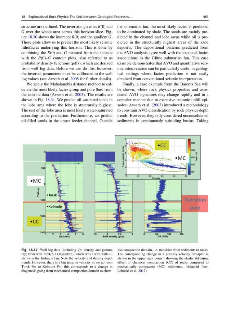
Fig. 18.32 Well log data (including Vp, density and gamma
ray) from well 7201/2-1 (Myrsildre), which was a well with oil
shows in the Kolmule Fm. Note the velocity and density depth
trends. However, there is a big jump in velocity as we go from
Torsk Fm to Kolmule Fm; this corresponds to a change in
diagenesis going from mechanical compaction domain to chemical compaction domain, i.e. transition from sediments to rocks.
The corresponding change in a porosity-velocity crossplot is
shown in the upper right corner, showing the elastic stiffening
effect of chemical compaction (CC) of rocks compared to
mechanically compacted (MC) sediments. (Adapted from
Lehocki et al. 2012)
18 Explorational Rock Physics: The Link between Geological Processes. . .
483
G over the whole area across this horizon slice. Figure 18.30 shows the intercept R(0) and the gradient G.
These plots allow us to predict the most likely seismic
lithofacies underlying this horizon. This is done by
combining the R(0) and G inverted from the seismic
with the R(0)–G contour plots, also referred to as
probability density functions (pdfs), which are derived
from well log data. Before we can do this, however,
the inverted parameters must be calibrated to the well
log values (see Avseth et al. 2005 for further details).
We apply the Mahalanobis distance method to calculate the most likely facies group and pore fluid from
the seismic data (Avseth et al. 2005). The results are
shown in Fig. 18.31. We predict oil-saturated sands in
the lobe area where the lobe is structurally highest.
The rest of the lobe area is most likely water-saturated
according to the prediction. Furthermore, we predict
oil-filled sands in the upper feeder-channel. Outside
the submarine fan, the most likely facies is predicted
to be dominated by shale. The sands are mainly predicted in the channel and lobe areas while oil is predicted in the structurally highest areas of the sand
deposits. The depositional patterns predicted from
the AVO analysis agree well with the expected facies
associations in the Glitne submarine fan. This case
example demonstrates that AVO and quantitative seismic interpretation can be particularly useful in geological settings where facies prediction is not easily
obtained from conventional seismic interpretation.
Finally, a case example from the Barents Sea will
be shown, where rock physics properties and associated AVO signatures may change rapidly and in a
complex manner due to extensive tectonic uplift episodes. Avseth et al. (2003) introduced a methodology
to constrain AVO classification by rock physics depth
trends. However, they only considered unconsolidated
sediments in continuously subsiding basins. Taking
Fig. 18.32 Well log data (including Vp, density and gamma
ray) from well 7201/2-1 (Myrsildre), which was a well with oil
shows in the Kolmule Fm. Note the velocity and density depth
trends. However, there is a big jump in velocity as we go from
Torsk Fm to Kolmule Fm; this corresponds to a change in
diagenesis going from mechanical compaction domain to chemical compaction domain, i.e. transition from sediments to rocks.
The corresponding change in a porosity-velocity crossplot is
shown in the upper right corner, showing the elastic stiffening
effect of chemical compaction (CC) of rocks compared to
mechanically compacted (MC) sediments. (Adapted from
Lehocki et al. 2012)
18 Explorational Rock Physics: The Link between Geological Processes. . .
483