

one reason why AVO analysis, used alone, can give
misleading results. In addition, these crossplots are
often affected by noise in the seismic data. Nevertheless, as we see in Fig. 18.27, we often observe that we
need both intercept (R(0)) and gradient (G) in order to
separate facies and fluid types from seismic data. Or
put another way, we often need to do AVO to discriminate lithology from fluids on seismic data.
Avseth et al. (2001a) applied the contour plots in
Fig. 18.27 to conduct an AVO analysis and predict
seismic lithofacies and pore fluids from the pre-stack
seismic amplitudes in the Glitne Field which are
depicted in the amplitude map in Fig. 18.1. As demonstrated in Fig. 18.1, the depositional trends in the
Glitne turbidite system do affect the seismic amplitudes. This is also confirmed by deterministic AVO
analysis of CDP gathers (see Fig. 18.28) at the three
well locations depicted in Fig. 18.1. The dramatic
variability in the lateral facies distribution, going
from a relatively proximal feeder-channel environment to a relatively distal lobe and lobe margin environment, has great impact on the seismic signatures in
this turbidite system.
The next step is facies and pore fluid prediction
from 3D seismic data. 3D AVO inversion is performed
on the turbidite system using Hampson-Russell’s
AVO software. Again, we focus only on the horizon
representing the top of the system (Top Heimdal).
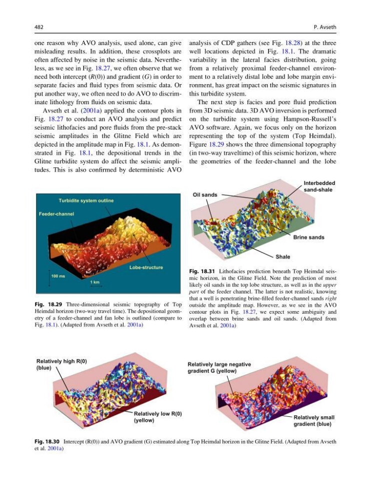
Figure 18.29 shows the three dimensional topography
(in two-way traveltime) of this seismic horizon, where
the geometries of the feeder-channel and the lobe
Feeder-channel
Lobe-structure
1 km
100 ms
Turbidite system outline
Fig. 18.29 Three-dimensional seismic topography of Top
Heimdal horizon (two-way travel time). The depositional geometry of a feeder-channel and fan lobe is outlined (compare to
Fig. 18.1). (Adapted from Avseth et al. 2001a)
Relatively high R(0)
(blue)
Relatively low R(0)
(yellow)
Relatively large negative
gradient G (yellow)
Relatively small
gradient (blue)
Fig. 18.30 Intercept (R(0)) and AVO gradient (G) estimated along Top Heimdal horizon in the Glitne Field. (Adapted from Avseth
et al. 2001a)
Oil sands
Shale
Brine sands
Interbedded
sand-shale
Fig. 18.31 Lithofacies prediction beneath Top Heimdal seismic horizon, in the Glitne Field. Note the prediction of most
likely oil sands in the top lobe structure, as well as in the upper
part of the feeder channel. The latter is not realistic, knowing
that a well is penetrating brine-filled feeder-channel sands right
outside the amplitude map. However, as we see in the AVO
contour plots in Fig. 18.27, we expect some ambiguity and
overlap between brine sands and oil sands. (Adapted from
Avseth et al. 2001a)
482
P. Avseth
misleading results. In addition, these crossplots are
often affected by noise in the seismic data. Nevertheless, as we see in Fig. 18.27, we often observe that we
need both intercept (R(0)) and gradient (G) in order to
separate facies and fluid types from seismic data. Or
put another way, we often need to do AVO to discriminate lithology from fluids on seismic data.
Avseth et al. (2001a) applied the contour plots in
Fig. 18.27 to conduct an AVO analysis and predict
seismic lithofacies and pore fluids from the pre-stack
seismic amplitudes in the Glitne Field which are
depicted in the amplitude map in Fig. 18.1. As demonstrated in Fig. 18.1, the depositional trends in the
Glitne turbidite system do affect the seismic amplitudes. This is also confirmed by deterministic AVO
analysis of CDP gathers (see Fig. 18.28) at the three
well locations depicted in Fig. 18.1. The dramatic
variability in the lateral facies distribution, going
from a relatively proximal feeder-channel environment to a relatively distal lobe and lobe margin environment, has great impact on the seismic signatures in
this turbidite system.
The next step is facies and pore fluid prediction
from 3D seismic data. 3D AVO inversion is performed
on the turbidite system using Hampson-Russell’s
AVO software. Again, we focus only on the horizon
representing the top of the system (Top Heimdal).
Figure 18.29 shows the three dimensional topography
(in two-way traveltime) of this seismic horizon, where
the geometries of the feeder-channel and the lobe
Feeder-channel
Lobe-structure
1 km
100 ms
Turbidite system outline
Fig. 18.29 Three-dimensional seismic topography of Top
Heimdal horizon (two-way travel time). The depositional geometry of a feeder-channel and fan lobe is outlined (compare to
Fig. 18.1). (Adapted from Avseth et al. 2001a)
Relatively high R(0)
(blue)
Relatively low R(0)
(yellow)
Relatively large negative
gradient G (yellow)
Relatively small
gradient (blue)
Fig. 18.30 Intercept (R(0)) and AVO gradient (G) estimated along Top Heimdal horizon in the Glitne Field. (Adapted from Avseth
et al. 2001a)
Oil sands
Shale
Brine sands
Interbedded
sand-shale
Fig. 18.31 Lithofacies prediction beneath Top Heimdal seismic horizon, in the Glitne Field. Note the prediction of most
likely oil sands in the top lobe structure, as well as in the upper
part of the feeder channel. The latter is not realistic, knowing
that a well is penetrating brine-filled feeder-channel sands right
outside the amplitude map. However, as we see in the AVO
contour plots in Fig. 18.27, we expect some ambiguity and
overlap between brine sands and oil sands. (Adapted from
Avseth et al. 2001a)
482
P. Avseth