

combinations of rock properties will yield the same
R(0) and G. Moreover, due to natural variability in
geological and fluid parameters, one given geological
scenario may span a relatively large possible outcome
area in the AVO crossplot, not just a discrete point.
Hence, a hydrocarbon-like AVO response might occasionally result from a brine-associated reflection, and
hydrocarbon-saturated sands might not always produce an anomalous AVO response; this problem was
seen in the RPT crossplots in Fig. 18.18. One way to
resolve this uncertainty is to create probability crossplots of various categories of lithology and pore fluid
scenarios. These can be based on statistical analysis of
well log data and/or rock physics models (Avseth
2000, Avseth et al. 2001a, b; Mukerji et al. 2001).
Each category is plotted as a “contour map”, almost
like topographical maps (Fig. 18.27). Here, the
“mountain tops” represent the most likely location of
a given class. It is very important to be aware that the
contours of different facies and fluids are overlapping
each other. This implies that an observed set of R(0)
and G can represent more than one category. This is
Cemented
trend
Clay
trend
Fluid
trend
Fig. 18.27 AVO contour plots or probability density functions
(pdfs) for main facies and fluids in the Glitne field. Only the isoprobability contours of 50% and larger are included for each
group. The R(0) and G pdfs nicely separate the three facies
groups, but there are significant overlaps. (Adapted from Avseth
et al. 2001a)
Top facies IIa
Top facies IIb
Top facies III
CDP
off
2000
2100
2200
2300
1
0 323 726 1210 1694 2177
CDP
off
CDP
off
2000
2100
2200
2300
2000
2100
2200
2300
1
1
0
0 323 726 1210 1694 2177
258 581 903 1226 1613 2000
Well # 1
Reflectivity
Reflectivity
Reflectivity
0.100
0.050
0
0.100
0.050
–0.050
–0.100
–0.150
–0.200
PR
PR
PR
0
0.100
0.050
–0.050
–0.100
0
–0.050
–0.100
Offset
angle
0
0
7
14
21
28
34 (deg)
500 1000 1500 2000 2500 (m)
Offset
angle
0
0
8
15
22
29 (deg)
500
1000
1500
2000 (m)
Offset
angle
0
0
7
14
20
26
(deg)
500 1000 1500 2000
32
2500 (m)
Well # 2
Well # 3
Well # 1
1900
2000
2100
2200
2300
1900
2000
2100
2200
2300
1900
2000
2100
2200
2300
Well # 2
Well # 3
Top_heimdal
Top_heimdal
Top_heimdal
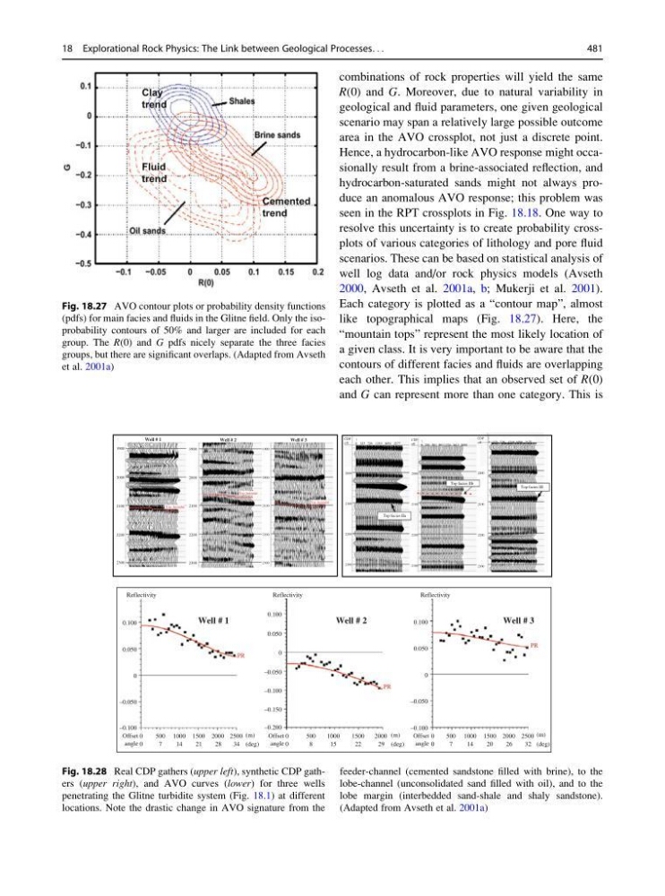
Fig. 18.28 Real CDP gathers (upper left), synthetic CDP gathers (upper right), and AVO curves (lower) for three wells
penetrating the Glitne turbidite system (Fig. 18.1) at different
locations. Note the drastic change in AVO signature from the
feeder-channel (cemented sandstone filled with brine), to the
lobe-channel (unconsolidated sand filled with oil), and to the
lobe margin (interbedded sand-shale and shaly sandstone).
(Adapted from Avseth et al. 2001a)
18 Explorational Rock Physics: The Link between Geological Processes. . .
481
R(0) and G. Moreover, due to natural variability in
geological and fluid parameters, one given geological
scenario may span a relatively large possible outcome
area in the AVO crossplot, not just a discrete point.
Hence, a hydrocarbon-like AVO response might occasionally result from a brine-associated reflection, and
hydrocarbon-saturated sands might not always produce an anomalous AVO response; this problem was
seen in the RPT crossplots in Fig. 18.18. One way to
resolve this uncertainty is to create probability crossplots of various categories of lithology and pore fluid
scenarios. These can be based on statistical analysis of
well log data and/or rock physics models (Avseth
2000, Avseth et al. 2001a, b; Mukerji et al. 2001).
Each category is plotted as a “contour map”, almost
like topographical maps (Fig. 18.27). Here, the
“mountain tops” represent the most likely location of
a given class. It is very important to be aware that the
contours of different facies and fluids are overlapping
each other. This implies that an observed set of R(0)
and G can represent more than one category. This is
Cemented
trend
Clay
trend
Fluid
trend
Fig. 18.27 AVO contour plots or probability density functions
(pdfs) for main facies and fluids in the Glitne field. Only the isoprobability contours of 50% and larger are included for each
group. The R(0) and G pdfs nicely separate the three facies
groups, but there are significant overlaps. (Adapted from Avseth
et al. 2001a)
Top facies IIa
Top facies IIb
Top facies III
CDP
off
2000
2100
2200
2300
1
0 323 726 1210 1694 2177
CDP
off
CDP
off
2000
2100
2200
2300
2000
2100
2200
2300
1
1
0
0 323 726 1210 1694 2177
258 581 903 1226 1613 2000
Well # 1
Reflectivity
Reflectivity
Reflectivity
0.100
0.050
0
0.100
0.050
–0.050
–0.100
–0.150
–0.200
PR
PR
PR
0
0.100
0.050
–0.050
–0.100
0
–0.050
–0.100
Offset
angle
0
0
7
14
21
28
34 (deg)
500 1000 1500 2000 2500 (m)
Offset
angle
0
0
8
15
22
29 (deg)
500
1000
1500
2000 (m)
Offset
angle
0
0
7
14
20
26
(deg)
500 1000 1500 2000
32
2500 (m)
Well # 2
Well # 3
Well # 1
1900
2000
2100
2200
2300
1900
2000
2100
2200
2300
1900
2000
2100
2200
2300
Well # 2
Well # 3
Top_heimdal
Top_heimdal
Top_heimdal
Fig. 18.28 Real CDP gathers (upper left), synthetic CDP gathers (upper right), and AVO curves (lower) for three wells
penetrating the Glitne turbidite system (Fig. 18.1) at different
locations. Note the drastic change in AVO signature from the
feeder-channel (cemented sandstone filled with brine), to the
lobe-channel (unconsolidated sand filled with oil), and to the
lobe margin (interbedded sand-shale and shaly sandstone).
(Adapted from Avseth et al. 2001a)
18 Explorational Rock Physics: The Link between Geological Processes. . .
481