

R θ
ð Þ % R 0
ð Þ þ G Á sin
2
θ
þ F tan
2
θ À sin
2
θ
À
Á
;
ð18:22Þ
where
R 0
ð Þ ¼
1
2
ΔV P
V P
þ
Δρ
ρ
;
G ¼
1
2
ΔV P
V P
À 2
V
2
S
V
2
P
Δρ
ρ
þ 2
ΔV S
V S
¼ R 0
ð Þ À
Δρ
ρ
1
2
þ
2V S
2
V P
2
À
4V S
2
V P
2
ΔV S
V S
;
and
F ¼
1
2
ΔV P
V P
:
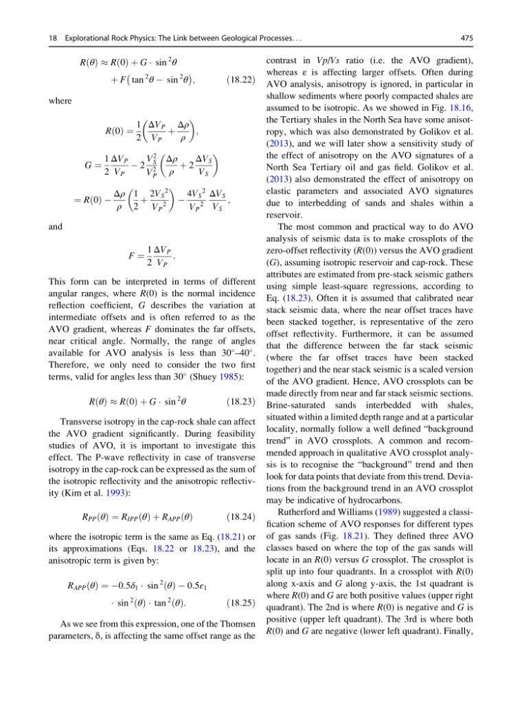
This form can be interpreted in terms of different
angular ranges, where R(0) is the normal incidence
reflection coefficient, G describes the variation at
intermediate offsets and is often referred to as the
AVO gradient, whereas F dominates the far offsets,
near critical angle. Normally, the range of angles
available for AVO analysis is less than 30
–40
.
Therefore, we only need to consider the two first
terms, valid for angles less than 30
(Shuey 1985):
R θ
ð Þ % R 0
ð Þ þ G Á sin
2
θ
ð18:23Þ
Transverse isotropy in the cap-rock shale can affect
the AVO gradient significantly. During feasibility
studies of AVO, it is important to investigate this
effect. The P-wave reflectivity in case of transverse
isotropy in the cap-rock can be expressed as the sum of
the isotropic reflectivity and the anisotropic reflectivity (Kim et al. 1993):
R PP θ
ð Þ ¼ R IPP θ
ð Þ þ R APP θ
ð Þ
ð18:24Þ
where the isotropic term is the same as Eq. (18.21) or
its approximations (Eqs. 18.22 or 18.23), and the
anisotropic term is given by:
R APP θ
ð Þ ¼ À0:5δ 1 Á sin
2
θ
ð Þ À 0:5ε 1
Á sin
2
θ
ð Þ Á tan
2
θ
ð Þ:
ð18:25Þ
As we see from this expression, one of the Thomsen
parameters, δ, is affecting the same offset range as the
contrast in Vp/Vs ratio (i.e. the AVO gradient),
whereas ε is affecting larger offsets. Often during
AVO analysis, anisotropy is ignored, in particular in
shallow sediments where poorly compacted shales are
assumed to be isotropic. As we showed in Fig. 18.16,
the Tertiary shales in the North Sea have some anisotropy, which was also demonstrated by Golikov et al.
(2013), and we will later show a sensitivity study of
the effect of anisotropy on the AVO signatures of a
North Sea Tertiary oil and gas field. Golikov et al.
(2013) also demonstrated the effect of anisotropy on
elastic parameters and associated AVO signatures
due to interbedding of sands and shales within a
reservoir.
The most common and practical way to do AVO
analysis of seismic data is to make crossplots of the
zero-offset reflectivity (R(0)) versus the AVO gradient
(G), assuming isotropic reservoir and cap-rock. These
attributes are estimated from pre-stack seismic gathers
using simple least-square regressions, according to
Eq. (18.23). Often it is assumed that calibrated near
stack seismic data, where the near offset traces have
been stacked together, is representative of the zero
offset reflectivity. Furthermore, it can be assumed
that the difference between the far stack seismic
(where the far offset traces have been stacked
together) and the near stack seismic is a scaled version
of the AVO gradient. Hence, AVO crossplots can be
made directly from near and far stack seismic sections.
Brine-saturated sands interbedded with shales,
situated within a limited depth range and at a particular
locality, normally follow a well defined “background
trend” in AVO crossplots. A common and recommended approach in qualitative AVO crossplot analysis is to recognise the “background” trend and then
look for data points that deviate from this trend. Deviations from the background trend in an AVO crossplot
may be indicative of hydrocarbons.
Rutherford and Williams (1989) suggested a classification scheme of AVO responses for different types
of gas sands (Fig. 18.21). They defined three AVO
classes based on where the top of the gas sands will
locate in an R(0) versus G crossplot. The crossplot is
split up into four quadrants. In a crossplot with R(0)
along x-axis and G along y-axis, the 1st quadrant is
where R(0) and G are both positive values (upper right
quadrant). The 2nd is where R(0) is negative and G is
positive (upper left quadrant). The 3rd is where both
R(0) and G are negative (lower left quadrant). Finally,
18 Explorational Rock Physics: The Link between Geological Processes. . .
475
ð Þ % R 0
ð Þ þ G Á sin
2
θ
þ F tan
2
θ À sin
2
θ
À
Á
;
ð18:22Þ
where
R 0
ð Þ ¼
1
2
ΔV P
V P
þ
Δρ
ρ
;
G ¼
1
2
ΔV P
V P
À 2
V
2
S
V
2
P
Δρ
ρ
þ 2
ΔV S
V S
¼ R 0
ð Þ À
Δρ
ρ
1
2
þ
2V S
2
V P
2
À
4V S
2
V P
2
ΔV S
V S
;
and
F ¼
1
2
ΔV P
V P
:
This form can be interpreted in terms of different
angular ranges, where R(0) is the normal incidence
reflection coefficient, G describes the variation at
intermediate offsets and is often referred to as the
AVO gradient, whereas F dominates the far offsets,
near critical angle. Normally, the range of angles
available for AVO analysis is less than 30
–40
.
Therefore, we only need to consider the two first
terms, valid for angles less than 30
(Shuey 1985):
R θ
ð Þ % R 0
ð Þ þ G Á sin
2
θ
ð18:23Þ
Transverse isotropy in the cap-rock shale can affect
the AVO gradient significantly. During feasibility
studies of AVO, it is important to investigate this
effect. The P-wave reflectivity in case of transverse
isotropy in the cap-rock can be expressed as the sum of
the isotropic reflectivity and the anisotropic reflectivity (Kim et al. 1993):
R PP θ
ð Þ ¼ R IPP θ
ð Þ þ R APP θ
ð Þ
ð18:24Þ
where the isotropic term is the same as Eq. (18.21) or
its approximations (Eqs. 18.22 or 18.23), and the
anisotropic term is given by:
R APP θ
ð Þ ¼ À0:5δ 1 Á sin
2
θ
ð Þ À 0:5ε 1
Á sin
2
θ
ð Þ Á tan
2
θ
ð Þ:
ð18:25Þ
As we see from this expression, one of the Thomsen
parameters, δ, is affecting the same offset range as the
contrast in Vp/Vs ratio (i.e. the AVO gradient),
whereas ε is affecting larger offsets. Often during
AVO analysis, anisotropy is ignored, in particular in
shallow sediments where poorly compacted shales are
assumed to be isotropic. As we showed in Fig. 18.16,
the Tertiary shales in the North Sea have some anisotropy, which was also demonstrated by Golikov et al.
(2013), and we will later show a sensitivity study of
the effect of anisotropy on the AVO signatures of a
North Sea Tertiary oil and gas field. Golikov et al.
(2013) also demonstrated the effect of anisotropy on
elastic parameters and associated AVO signatures
due to interbedding of sands and shales within a
reservoir.
The most common and practical way to do AVO
analysis of seismic data is to make crossplots of the
zero-offset reflectivity (R(0)) versus the AVO gradient
(G), assuming isotropic reservoir and cap-rock. These
attributes are estimated from pre-stack seismic gathers
using simple least-square regressions, according to
Eq. (18.23). Often it is assumed that calibrated near
stack seismic data, where the near offset traces have
been stacked together, is representative of the zero
offset reflectivity. Furthermore, it can be assumed
that the difference between the far stack seismic
(where the far offset traces have been stacked
together) and the near stack seismic is a scaled version
of the AVO gradient. Hence, AVO crossplots can be
made directly from near and far stack seismic sections.
Brine-saturated sands interbedded with shales,
situated within a limited depth range and at a particular
locality, normally follow a well defined “background
trend” in AVO crossplots. A common and recommended approach in qualitative AVO crossplot analysis is to recognise the “background” trend and then
look for data points that deviate from this trend. Deviations from the background trend in an AVO crossplot
may be indicative of hydrocarbons.
Rutherford and Williams (1989) suggested a classification scheme of AVO responses for different types
of gas sands (Fig. 18.21). They defined three AVO
classes based on where the top of the gas sands will
locate in an R(0) versus G crossplot. The crossplot is
split up into four quadrants. In a crossplot with R(0)
along x-axis and G along y-axis, the 1st quadrant is
where R(0) and G are both positive values (upper right
quadrant). The 2nd is where R(0) is negative and G is
positive (upper left quadrant). The 3rd is where both
R(0) and G are negative (lower left quadrant). Finally,
18 Explorational Rock Physics: The Link between Geological Processes. . .
475