

prediction in many areas of the world, yet in some
cases it failed. The technique suffered from ambiguities caused by lithological effects, tuning effects and
overburden effects. It turned out that even seismic
processing and acquisition effects could cause false
AVO anomalies. Application of AVO analysis was
therefore reduced. However, in many of these cases
it was incorrect use of the technique that was responsible for the failure, not the technique itself. In the last
decade we have observed a revival of the AVO technique. This is due to the improvement of 3D seismic
technology, better pre-processing routines, more frequent shear-wave logging that can better constrain
AVO modelling, improved understanding of rock
physics properties, greater data capacity, more focus
on cross-disciplinary aspects of AVO and, last but not
least, more awareness among the users of the potential
pitfalls.
The technique provides the seismic interpreter with
information about pore fluids and lithologies, which
complements the conventional interpretation of seismic facies, stratigraphy and geomorphology. The
reflection coefficient for plane elastic waves as a function of reflection angle at a single interface, also
referred to as the AVO response, is described by the
complicated Zoeppritz equations (Zoeppritz 1919).
For analysis of P-wave reflections, a well-known
approximation is given by Aki and Richards (1980),
assuming weak layer contrasts:
R θ 1
ð Þ %
1
2
1 À 4p
2 V
2
s
À
Á Δρ
ρ
þ
1
2 cos 2 θ
ΔV p
V p
À 4p
2 V
2
S
ΔV S
V S
;
ð18:21Þ
where:
p ¼
sin θ 1
V P1
θ ¼ θ 1 þ θ 2
ð
Þ=2 % θ 1
Δρ ¼ ρ 2 À ρ 1 ρ ¼ ρ 2 þ ρ 1
ð
Þ =2
ΔV P ¼ V P2 À V P1 V P ¼ V P2 þ V P1
ð
Þ =2
ΔV S ¼ V S2 À V S1 V S ¼ V S2 þ V S1
ð
Þ =2
In the formulae above, p is the ray parameter, θ 1 is
the angle of incidence, and θ 2 is the transmission
angle. V P1 and V P2 are the P-wave velocities above
and below a given interface, respectively. Similarly,
V S1 and V S2 are the S-wave velocities, while ρ 1 and
ρ 2 are densities above and below this interface.
The approximation given by Aki and Richards can
be further approximated (Shuey 1985):
Stack section
CDP GATHER
AVO response at target
horizon
Geological interpretation
Shale
Sandstone
with gas
Offset (or angle
of incidence)
Time
Reflectivity
0.15
0.1
0.05
0
–0.05
–0.1
–0.15
–0.2
–0.25
0 5 10 15 20 25 30 35
angle of incidence
40
Time
CDP
location
Target horizon
Target horizon
CDP gather
of interest
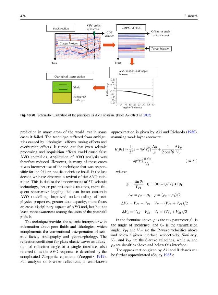
Fig. 18.20 Schematic illustration of the principles in AVO analysis. (From Avseth et al. 2005)
474
P. Avseth
cases it failed. The technique suffered from ambiguities caused by lithological effects, tuning effects and
overburden effects. It turned out that even seismic
processing and acquisition effects could cause false
AVO anomalies. Application of AVO analysis was
therefore reduced. However, in many of these cases
it was incorrect use of the technique that was responsible for the failure, not the technique itself. In the last
decade we have observed a revival of the AVO technique. This is due to the improvement of 3D seismic
technology, better pre-processing routines, more frequent shear-wave logging that can better constrain
AVO modelling, improved understanding of rock
physics properties, greater data capacity, more focus
on cross-disciplinary aspects of AVO and, last but not
least, more awareness among the users of the potential
pitfalls.
The technique provides the seismic interpreter with
information about pore fluids and lithologies, which
complements the conventional interpretation of seismic facies, stratigraphy and geomorphology. The
reflection coefficient for plane elastic waves as a function of reflection angle at a single interface, also
referred to as the AVO response, is described by the
complicated Zoeppritz equations (Zoeppritz 1919).
For analysis of P-wave reflections, a well-known
approximation is given by Aki and Richards (1980),
assuming weak layer contrasts:
R θ 1
ð Þ %
1
2
1 À 4p
2 V
2
s
À
Á Δρ
ρ
þ
1
2 cos 2 θ
ΔV p
V p
À 4p
2 V
2
S
ΔV S
V S
;
ð18:21Þ
where:
p ¼
sin θ 1
V P1
θ ¼ θ 1 þ θ 2
ð
Þ=2 % θ 1
Δρ ¼ ρ 2 À ρ 1 ρ ¼ ρ 2 þ ρ 1
ð
Þ =2
ΔV P ¼ V P2 À V P1 V P ¼ V P2 þ V P1
ð
Þ =2
ΔV S ¼ V S2 À V S1 V S ¼ V S2 þ V S1
ð
Þ =2
In the formulae above, p is the ray parameter, θ 1 is
the angle of incidence, and θ 2 is the transmission
angle. V P1 and V P2 are the P-wave velocities above
and below a given interface, respectively. Similarly,
V S1 and V S2 are the S-wave velocities, while ρ 1 and
ρ 2 are densities above and below this interface.
The approximation given by Aki and Richards can
be further approximated (Shuey 1985):
Stack section
CDP GATHER
AVO response at target
horizon
Geological interpretation
Shale
Sandstone
with gas
Offset (or angle
of incidence)
Time
Reflectivity
0.15
0.1
0.05
0
–0.05
–0.1
–0.15
–0.2
–0.25
0 5 10 15 20 25 30 35
angle of incidence
40
Time
CDP
location
Target horizon
Target horizon
CDP gather
of interest
Fig. 18.20 Schematic illustration of the principles in AVO analysis. (From Avseth et al. 2005)
474
P. Avseth