

seismic wave period results in a stiffer effective rock
than is the case with uniform saturation where the
fluids have time to equilibrate.
Equation (18.20) appears to be an upper bound, and
data seldom fall on it, except at very low gas saturations.
18.7 Rock Physics Templates
We can combine the depositional and diagenetic trend
models presented above with Gassmann fluid substitution, and make charts or templates of rock physics
models for predicting lithology and presence of hydrocarbons. We refer to these locally constrained charts as
Rock Physics Templates (RPTs), a methodology first
presented by Ødegaard and Avseth (2004). Furthermore, we expand on the rock physics diagnostics presented earlier as we create RPTs of seismic parameters,
in our case acoustic impedance (AI ¼ V P Á ρ) versus
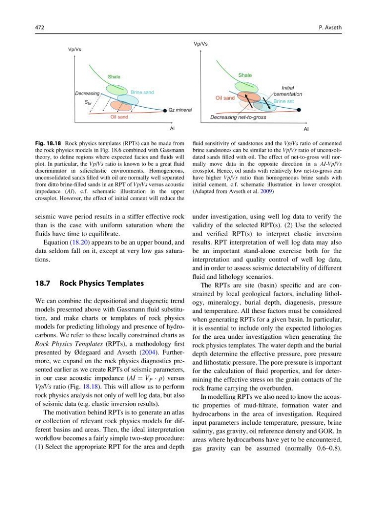
Vp/Vs ratio (Fig. 18.18). This will allow us to perform
rock physics analysis not only of well log data, but also
of seismic data (e.g. elastic inversion results).
The motivation behind RPTs is to generate an atlas
or collection of relevant rock physics models for different basins and areas. Then, the ideal interpretation
workflow becomes a fairly simple two-step procedure:
(1) Select the appropriate RPT for the area and depth
under investigation, using well log data to verify the
validity of the selected RPT(s). (2) Use the selected
and verified RPT(s) to interpret elastic inversion
results. RPT interpretation of well log data may also
be an important stand-alone exercise both for the
interpretation and quality control of well log data,
and in order to assess seismic detectability of different
fluid and lithology scenarios.
The RPTs are site (basin) specific and are constrained by local geological factors, including lithology, mineralogy, burial depth, diagenesis, pressure
and temperature. All these factors must be considered
when generating RPTs for a given basin. In particular,
it is essential to include only the expected lithologies
for the area under investigation when generating the
rock physics templates. The water depth and the burial
depth determine the effective pressure, pore pressure
and lithostatic pressure. The pore pressure is important
for the calculation of fluid properties, and for determining the effective stress on the grain contacts of the
rock frame carrying the overburden.
In modelling RPTs we also need to know the acoustic properties of mud-filtrate, formation water and
hydrocarbons in the area of investigation. Required
input parameters include temperature, pressure, brine
salinity, gas gravity, oil reference density and GOR. In
areas where hydrocarbons have yet to be encountered,
gas gravity can be assumed (normally 0.6–0.8).
Vp/Vs
AI
Shale
Brine sand
Oil sand
Qz mineral
Decreasing
S br
Vp/Vs
AI
Oil sand
Shale
Brine sst
Initial
cementation
Decreasing net-to-gross
Fig. 18.18 Rock physics templates (RPTs) can be made from
the rock physics models in Fig. 18.6 combined with Gassmann
theory, to define regions where expected facies and fluids will
plot. In particular, the Vp/Vs ratio is known to be a great fluid
discriminator in siliciclastic environments. Homogeneous,
unconsolidated sands filled with oil are normally well separated
from ditto brine-filled sands in an RPT of Vp/Vs versus acoustic
impedance (AI), c.f. schematic illustration in the upper
crossplot. However, the effect of initial cement will reduce the
fluid sensitivity of sandstones and the Vp/Vs ratio of cemented
brine sandstones can be similar to the Vp/Vs ratio of unconsolidated sands filled with oil. The effect of net-to-gross will normally move data in the opposite direction in a AI-Vp/Vs
crossplot. Hence, oil sands with relatively low net-to-gross can
have higher Vp/Vs ratio than homogeneous brine sands with
initial cement, c.f. schematic illustration in lower crossplot.
(Adapted from Avseth et al. 2009)
472
P. Avseth
than is the case with uniform saturation where the
fluids have time to equilibrate.
Equation (18.20) appears to be an upper bound, and
data seldom fall on it, except at very low gas saturations.
18.7 Rock Physics Templates
We can combine the depositional and diagenetic trend
models presented above with Gassmann fluid substitution, and make charts or templates of rock physics
models for predicting lithology and presence of hydrocarbons. We refer to these locally constrained charts as
Rock Physics Templates (RPTs), a methodology first
presented by Ødegaard and Avseth (2004). Furthermore, we expand on the rock physics diagnostics presented earlier as we create RPTs of seismic parameters,
in our case acoustic impedance (AI ¼ V P Á ρ) versus
Vp/Vs ratio (Fig. 18.18). This will allow us to perform
rock physics analysis not only of well log data, but also
of seismic data (e.g. elastic inversion results).
The motivation behind RPTs is to generate an atlas
or collection of relevant rock physics models for different basins and areas. Then, the ideal interpretation
workflow becomes a fairly simple two-step procedure:
(1) Select the appropriate RPT for the area and depth
under investigation, using well log data to verify the
validity of the selected RPT(s). (2) Use the selected
and verified RPT(s) to interpret elastic inversion
results. RPT interpretation of well log data may also
be an important stand-alone exercise both for the
interpretation and quality control of well log data,
and in order to assess seismic detectability of different
fluid and lithology scenarios.
The RPTs are site (basin) specific and are constrained by local geological factors, including lithology, mineralogy, burial depth, diagenesis, pressure
and temperature. All these factors must be considered
when generating RPTs for a given basin. In particular,
it is essential to include only the expected lithologies
for the area under investigation when generating the
rock physics templates. The water depth and the burial
depth determine the effective pressure, pore pressure
and lithostatic pressure. The pore pressure is important
for the calculation of fluid properties, and for determining the effective stress on the grain contacts of the
rock frame carrying the overburden.
In modelling RPTs we also need to know the acoustic properties of mud-filtrate, formation water and
hydrocarbons in the area of investigation. Required
input parameters include temperature, pressure, brine
salinity, gas gravity, oil reference density and GOR. In
areas where hydrocarbons have yet to be encountered,
gas gravity can be assumed (normally 0.6–0.8).
Vp/Vs
AI
Shale
Brine sand
Oil sand
Qz mineral
Decreasing
S br
Vp/Vs
AI
Oil sand
Shale
Brine sst
Initial
cementation
Decreasing net-to-gross
Fig. 18.18 Rock physics templates (RPTs) can be made from
the rock physics models in Fig. 18.6 combined with Gassmann
theory, to define regions where expected facies and fluids will
plot. In particular, the Vp/Vs ratio is known to be a great fluid
discriminator in siliciclastic environments. Homogeneous,
unconsolidated sands filled with oil are normally well separated
from ditto brine-filled sands in an RPT of Vp/Vs versus acoustic
impedance (AI), c.f. schematic illustration in the upper
crossplot. However, the effect of initial cement will reduce the
fluid sensitivity of sandstones and the Vp/Vs ratio of cemented
brine sandstones can be similar to the Vp/Vs ratio of unconsolidated sands filled with oil. The effect of net-to-gross will normally move data in the opposite direction in a AI-Vp/Vs
crossplot. Hence, oil sands with relatively low net-to-gross can
have higher Vp/Vs ratio than homogeneous brine sands with
initial cement, c.f. schematic illustration in lower crossplot.
(Adapted from Avseth et al. 2009)
472
P. Avseth