

monomineralic assumption, but an effective mineral
modulus can be approximated via the Hill’s average or
Hashin-Shtrikman modelling (see Mavko et al. 2009).
Another issue is whether the clay should be considered
only as part of the mineral frame, or should the bound
water that constitutes part of the clay mineral be considered part of the fluid when we do Gassmann fluid
substitution? If the latter, then the functional Gassmann porosity is actually larger than the total porosity,
but the pore fluid should be considered a muddy suspension containing clay particles.
Gassmann’s relations were originally derived to
describe the change in rock modulus from one pure
saturation to another – from dry to fully brinesaturated, from fully brine-saturated to fully oilsaturated, etc. Domenico (1976) suggested that
mixed gas-oil-brine saturations can also be modelled
with Gassmann’s relations, if the mixture of phases is
replaced with an effective fluid with bulk modulus
K fluid and density ρ fluid given by
1
K fluid
¼
S gas
K gas
þ
S oil
K oil
þ
S br
K br
¼
1
K fluid x; y; z
ð
Þ
(
)
ð18:18Þ
ρ fluid ¼ S gas ρ gas þ S oil ρ oil þ S br ρ br
¼ ρ fluid x; y; z
ð
Þ
ð18:19Þ
where S gas,oil,br, K gas,oil,br , and ρ gas,oil,br are the saturations, bulk moduli, and densities of the gas, oil, and
brine phases. The operator h Á i refers to a volume
average and allows for more compact expressions,
where K fluid (x, y, z) and ρ fluid (x, y, z) are the spatially
varying pore fluid modulus and density.
Substituting Eq. (18.18) into Gassmann’s relation is
the procedure most widely used today to model fluid
effects on seismic velocity and impedance for low
frequency field applications. The fluid properties are
obtained through the Batzle and Wang (1992) equations, and these normally comprise brine salinity, gas
gravity, oil reference density, gas/oil ratio (GOR),
temperature and pore pressure.
A problem with mixed fluid phases is that velocities
depend not only on saturations but also on the spatial
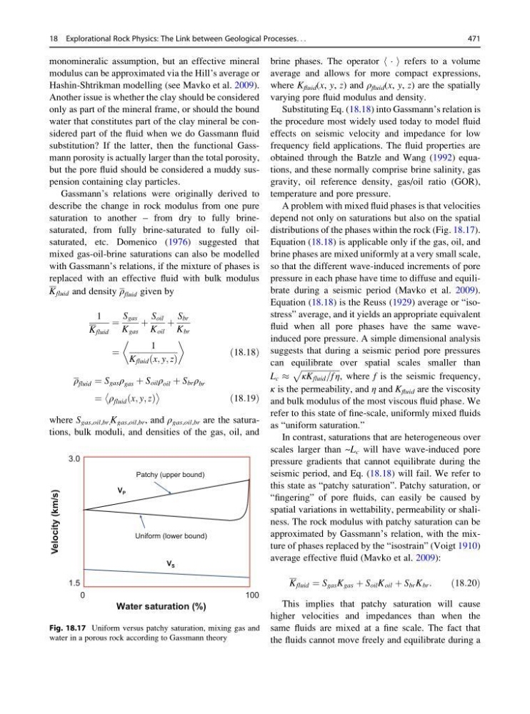
distributions of the phases within the rock (Fig. 18.17).
Equation (18.18) is applicable only if the gas, oil, and
brine phases are mixed uniformly at a very small scale,
so that the different wave-induced increments of pore
pressure in each phase have time to diffuse and equilibrate during a seismic period (Mavko et al. 2009).
Equation (18.18) is the Reuss (1929) average or “isostress” average, and it yields an appropriate equivalent
fluid when all pore phases have the same waveinduced pore pressure. A simple dimensional analysis
suggests that during a seismic period pore pressures
can equilibrate over spatial scales smaller than
L c %
ffiffiffiffiffiffiffiffiffiffiffiffiffiffiffiffiffiffiffi
κK fluid =f η
p
, where f is the seismic frequency,
κ is the permeability, and η and K fluid are the viscosity
and bulk modulus of the most viscous fluid phase. We
refer to this state of fine-scale, uniformly mixed fluids
as “uniform saturation.”
In contrast, saturations that are heterogeneous over
scales larger than ~L c will have wave-induced pore
pressure gradients that cannot equilibrate during the
seismic period, and Eq. (18.18) will fail. We refer to
this state as “patchy saturation”. Patchy saturation, or
“fingering” of pore fluids, can easily be caused by
spatial variations in wettability, permeability or shaliness. The rock modulus with patchy saturation can be
approximated by Gassmann’s relation, with the mixture of phases replaced by the “isostrain” (Voigt 1910)
average effective fluid (Mavko et al. 2009):
K fluid ¼ S gas K gas þ S oil K oil þ S br K br :
ð18:20Þ
This implies that patchy saturation will cause
higher velocities and impedances than when the
same fluids are mixed at a fine scale. The fact that
the fluids cannot move freely and equilibrate during a
Velocity (km/s)
0
Water saturation (%)
100
1.5
3.0
V S
V P
Patchy (upper bound)
Uniform (lower bound)
Fig. 18.17 Uniform versus patchy saturation, mixing gas and
water in a porous rock according to Gassmann theory
18 Explorational Rock Physics: The Link between Geological Processes. . .
471
modulus can be approximated via the Hill’s average or
Hashin-Shtrikman modelling (see Mavko et al. 2009).
Another issue is whether the clay should be considered
only as part of the mineral frame, or should the bound
water that constitutes part of the clay mineral be considered part of the fluid when we do Gassmann fluid
substitution? If the latter, then the functional Gassmann porosity is actually larger than the total porosity,
but the pore fluid should be considered a muddy suspension containing clay particles.
Gassmann’s relations were originally derived to
describe the change in rock modulus from one pure
saturation to another – from dry to fully brinesaturated, from fully brine-saturated to fully oilsaturated, etc. Domenico (1976) suggested that
mixed gas-oil-brine saturations can also be modelled
with Gassmann’s relations, if the mixture of phases is
replaced with an effective fluid with bulk modulus
K fluid and density ρ fluid given by
1
K fluid
¼
S gas
K gas
þ
S oil
K oil
þ
S br
K br
¼
1
K fluid x; y; z
ð
Þ
(
)
ð18:18Þ
ρ fluid ¼ S gas ρ gas þ S oil ρ oil þ S br ρ br
¼ ρ fluid x; y; z
ð
Þ
ð18:19Þ
where S gas,oil,br, K gas,oil,br , and ρ gas,oil,br are the saturations, bulk moduli, and densities of the gas, oil, and
brine phases. The operator h Á i refers to a volume
average and allows for more compact expressions,
where K fluid (x, y, z) and ρ fluid (x, y, z) are the spatially
varying pore fluid modulus and density.
Substituting Eq. (18.18) into Gassmann’s relation is
the procedure most widely used today to model fluid
effects on seismic velocity and impedance for low
frequency field applications. The fluid properties are
obtained through the Batzle and Wang (1992) equations, and these normally comprise brine salinity, gas
gravity, oil reference density, gas/oil ratio (GOR),
temperature and pore pressure.
A problem with mixed fluid phases is that velocities
depend not only on saturations but also on the spatial
distributions of the phases within the rock (Fig. 18.17).
Equation (18.18) is applicable only if the gas, oil, and
brine phases are mixed uniformly at a very small scale,
so that the different wave-induced increments of pore
pressure in each phase have time to diffuse and equilibrate during a seismic period (Mavko et al. 2009).
Equation (18.18) is the Reuss (1929) average or “isostress” average, and it yields an appropriate equivalent
fluid when all pore phases have the same waveinduced pore pressure. A simple dimensional analysis
suggests that during a seismic period pore pressures
can equilibrate over spatial scales smaller than
L c %
ffiffiffiffiffiffiffiffiffiffiffiffiffiffiffiffiffiffiffi
κK fluid =f η
p
, where f is the seismic frequency,
κ is the permeability, and η and K fluid are the viscosity
and bulk modulus of the most viscous fluid phase. We
refer to this state of fine-scale, uniformly mixed fluids
as “uniform saturation.”
In contrast, saturations that are heterogeneous over
scales larger than ~L c will have wave-induced pore
pressure gradients that cannot equilibrate during the
seismic period, and Eq. (18.18) will fail. We refer to
this state as “patchy saturation”. Patchy saturation, or
“fingering” of pore fluids, can easily be caused by
spatial variations in wettability, permeability or shaliness. The rock modulus with patchy saturation can be
approximated by Gassmann’s relation, with the mixture of phases replaced by the “isostrain” (Voigt 1910)
average effective fluid (Mavko et al. 2009):
K fluid ¼ S gas K gas þ S oil K oil þ S br K br :
ð18:20Þ
This implies that patchy saturation will cause
higher velocities and impedances than when the
same fluids are mixed at a fine scale. The fact that
the fluids cannot move freely and equilibrate during a
Velocity (km/s)
0
Water saturation (%)
100
1.5
3.0
V S
V P
Patchy (upper bound)
Uniform (lower bound)
Fig. 18.17 Uniform versus patchy saturation, mixing gas and
water in a porous rock according to Gassmann theory
18 Explorational Rock Physics: The Link between Geological Processes. . .
471