

where pores are poorly connected (e.g. Hornby et al.
1994, Johansen et al. 2002, Avseth et al. 2014), and
where contact theory and granular-based models presented above are not representative or valid. For shales
and heterogeneous sandstones it may be important to
take into account the anisotropy effect on seismic
velocities (e.g. Golikov et al. 2013). The sedimentological layering of interbedded sands and shales, and
the internal texture of shale, will yield transverse isotropy, where seismic waves propagating in the vertical
direction will travel at a slower velocity than seismic
waves propagating in the horizontal direction. In an
isotropic medium we are only dealing with two independent elastic constants as given in the isotropic
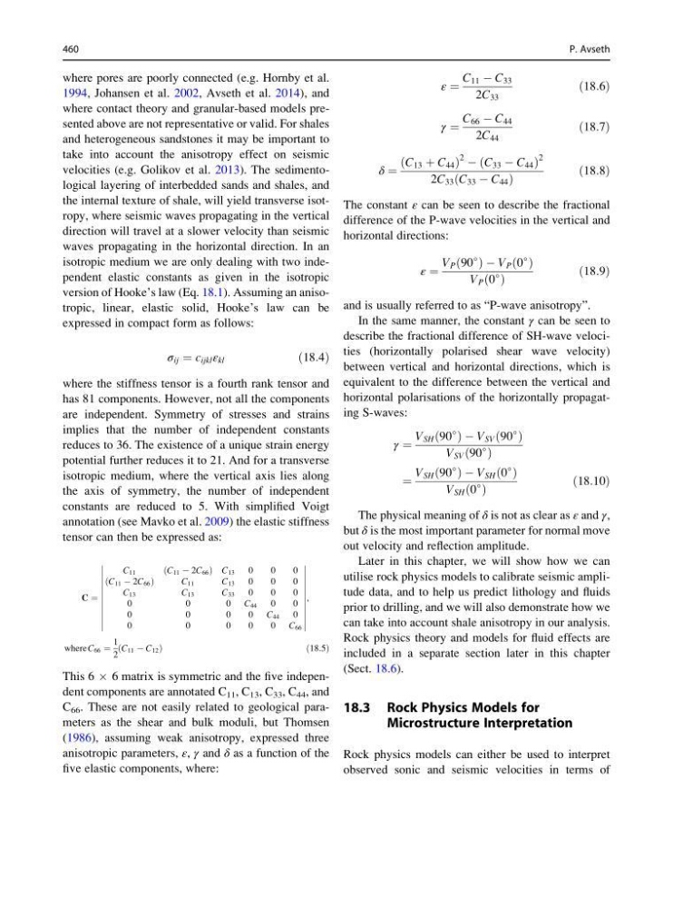
version of Hooke’s law (Eq. 18.1). Assuming an anisotropic, linear, elastic solid, Hooke’s law can be
expressed in compact form as follows:
σ ij ¼ c ijkl ε kl
ð18:4Þ
where the stiffness tensor is a fourth rank tensor and
has 81 components. However, not all the components
are independent. Symmetry of stresses and strains
implies that the number of independent constants
reduces to 36. The existence of a unique strain energy
potential further reduces it to 21. And for a transverse
isotropic medium, where the vertical axis lies along
the axis of symmetry, the number of independent
constants are reduced to 5. With simplified Voigt
annotation (see Mavko et al. 2009) the elastic stiffness
tensor can then be expressed as:
C ¼
C 11
C 11 À 2C 66
ð
Þ C 13
0
0
0
C 11 À 2C 66
ð
Þ
C 11
C 13
0
0
0
C 13
C 13
C 33
0
0
0
0
0
0 C 44
0
0
0
0
0
0 C 44
0
0
0
0
0
0 C 66
,
where C 66 ¼
1
2
C 11 À C 12
ð
Þ
ð18:5Þ
This 6 Â 6 matrix is symmetric and the five independent components are annotated C 11 , C 13 , C 33 , C 44 , and
C 66 . These are not easily related to geological parameters as the shear and bulk moduli, but Thomsen
(1986), assuming weak anisotropy, expressed three
anisotropic parameters, ε, γ and δ as a function of the
five elastic components, where:
ε ¼
C 11 À C 33
2C 33
ð18:6Þ
γ ¼
C 66 À C 44
2C 44
ð18:7Þ
δ ¼
C 13 þ C 44
ð
Þ
2 À C 33 À C 44
ð
Þ
2
2C 33 C 33 À C 44
ð
Þ
ð18:8Þ
The constant ε can be seen to describe the fractional
difference of the P-wave velocities in the vertical and
horizontal directions:
ε ¼
V P 90
∘
ð ÞÀV P 0
∘
ð Þ
V P 0
∘
ð Þ
ð18:9Þ
and is usually referred to as “P-wave anisotropy”.
In the same manner, the constant γ can be seen to
describe the fractional difference of SH-wave velocities (horizontally polarised shear wave velocity)
between vertical and horizontal directions, which is
equivalent to the difference between the vertical and
horizontal polarisations of the horizontally propagating S-waves:
γ ¼
V SH 90
∘
ð ÞÀV SV 90
∘
ð Þ
V SV 90
∘
ð Þ
¼
V SH 90
∘
ð ÞÀV SH 0
∘
ð Þ
V SH 0
∘
ð Þ
ð18:10Þ
The physical meaning of δ is not as clear as ε and γ,
but δ is the most important parameter for normal move
out velocity and reflection amplitude.
Later in this chapter, we will show how we can
utilise rock physics models to calibrate seismic amplitude data, and to help us predict lithology and fluids
prior to drilling, and we will also demonstrate how we
can take into account shale anisotropy in our analysis.
Rock physics theory and models for fluid effects are
included in a separate section later in this chapter
(Sect. 18.6).
18.3 Rock Physics Models for
Microstructure Interpretation
Rock physics models can either be used to interpret
observed sonic and seismic velocities in terms of
460
P. Avseth
1994, Johansen et al. 2002, Avseth et al. 2014), and
where contact theory and granular-based models presented above are not representative or valid. For shales
and heterogeneous sandstones it may be important to
take into account the anisotropy effect on seismic
velocities (e.g. Golikov et al. 2013). The sedimentological layering of interbedded sands and shales, and
the internal texture of shale, will yield transverse isotropy, where seismic waves propagating in the vertical
direction will travel at a slower velocity than seismic
waves propagating in the horizontal direction. In an
isotropic medium we are only dealing with two independent elastic constants as given in the isotropic
version of Hooke’s law (Eq. 18.1). Assuming an anisotropic, linear, elastic solid, Hooke’s law can be
expressed in compact form as follows:
σ ij ¼ c ijkl ε kl
ð18:4Þ
where the stiffness tensor is a fourth rank tensor and
has 81 components. However, not all the components
are independent. Symmetry of stresses and strains
implies that the number of independent constants
reduces to 36. The existence of a unique strain energy
potential further reduces it to 21. And for a transverse
isotropic medium, where the vertical axis lies along
the axis of symmetry, the number of independent
constants are reduced to 5. With simplified Voigt
annotation (see Mavko et al. 2009) the elastic stiffness
tensor can then be expressed as:
C ¼
C 11
C 11 À 2C 66
ð
Þ C 13
0
0
0
C 11 À 2C 66
ð
Þ
C 11
C 13
0
0
0
C 13
C 13
C 33
0
0
0
0
0
0 C 44
0
0
0
0
0
0 C 44
0
0
0
0
0
0 C 66
,
where C 66 ¼
1
2
C 11 À C 12
ð
Þ
ð18:5Þ
This 6 Â 6 matrix is symmetric and the five independent components are annotated C 11 , C 13 , C 33 , C 44 , and
C 66 . These are not easily related to geological parameters as the shear and bulk moduli, but Thomsen
(1986), assuming weak anisotropy, expressed three
anisotropic parameters, ε, γ and δ as a function of the
five elastic components, where:
ε ¼
C 11 À C 33
2C 33
ð18:6Þ
γ ¼
C 66 À C 44
2C 44
ð18:7Þ
δ ¼
C 13 þ C 44
ð
Þ
2 À C 33 À C 44
ð
Þ
2
2C 33 C 33 À C 44
ð
Þ
ð18:8Þ
The constant ε can be seen to describe the fractional
difference of the P-wave velocities in the vertical and
horizontal directions:
ε ¼
V P 90
∘
ð ÞÀV P 0
∘
ð Þ
V P 0
∘
ð Þ
ð18:9Þ
and is usually referred to as “P-wave anisotropy”.
In the same manner, the constant γ can be seen to
describe the fractional difference of SH-wave velocities (horizontally polarised shear wave velocity)
between vertical and horizontal directions, which is
equivalent to the difference between the vertical and
horizontal polarisations of the horizontally propagating S-waves:
γ ¼
V SH 90
∘
ð ÞÀV SV 90
∘
ð Þ
V SV 90
∘
ð Þ
¼
V SH 90
∘
ð ÞÀV SH 0
∘
ð Þ
V SH 0
∘
ð Þ
ð18:10Þ
The physical meaning of δ is not as clear as ε and γ,
but δ is the most important parameter for normal move
out velocity and reflection amplitude.
Later in this chapter, we will show how we can
utilise rock physics models to calibrate seismic amplitude data, and to help us predict lithology and fluids
prior to drilling, and we will also demonstrate how we
can take into account shale anisotropy in our analysis.
Rock physics theory and models for fluid effects are
included in a separate section later in this chapter
(Sect. 18.6).
18.3 Rock Physics Models for
Microstructure Interpretation
Rock physics models can either be used to interpret
observed sonic and seismic velocities in terms of
460
P. Avseth