

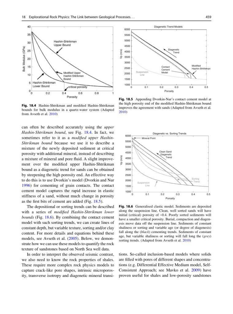
can often be described accurately using the upper
Hashin-Shtrikman bound, see Fig. 18.4. In fact, we
sometimes refer to it as a modified upper HashinShtrikman bound because we use it to describe a
mixture of the newly deposited sediment at critical
porosity with additional mineral, instead of describing
a mixture of mineral and pore fluid. A slight improvement over the modified upper Hashin-Shtrikman
bound as a diagenetic trend for sands can be obtained
by steepening the high porosity end. An effective way
to do this is to use Dvorkin’s model (Dvorkin and Nur
1996) for cementing of grain contacts. The contact
cement model captures the rapid increase in elastic
stiffness of a sand, without much change in porosity
as the first bits of cement are added (Fig. 18.5).
The depositional or sorting trends can be described
with a series of modified Hashin-Shtrikman lower
bounds (Fig. 18.6). By combining the contact cement
model with such sorting trends, we can create lines of
constant depth, but variable texture, sorting and/or clay
content. For more details and equations behind these
models, see Avseth et al. (2005). Below, we demonstrate how we can use these models to quantify the rock
texture of sandstones based on North Sea well data.
In order to interpret the observed seismic contrast,
we also need to know the rock properties of shales.
These require more complex rock physics models to
capture crack-like pore shapes, intrinsic microporosity, transverse isotropy and diagenetic mineral transitions. So-called inclusion-based models where solids
are filled with pores of different shapes and concentrations (e.g. Differential Effective Medium model, SelfConsistent Approach; see Mavko et al. 2009) have
proven useful for shales and low-porosity sandstones
Fig. 18.4 Hashin-Shtrikman and modified Hashin-Shtrikman
bounds for bulk modulus in a quartz-water system (Adapted
from Avseth et al. 2010)
Diagenetic Trend Models
Diagenetic
Trend
Modified
Hashin-Shtrikman
Contact
Cement
Model
Suspension
Line
Porosity
Vp (m/s)
6000
5500
5000
4500
4000
3500
3000
2500
2000
1500
1000
0
0.1
0.2
0.3
0.4
0.5
Fig. 18.5 Appending Dvorkin-Nur’s contact cement model at
the high porosity end of the modified Hashin-Shtrikman bound
improves the agreement with sands (Adapted from Avseth et al.
2010)
6000
Mineral Point
Clean Sand
Diagenetic
Trend
Suspension
Line
Sorting
Trend
Diagenetic vs. Sorting Trends
5500
5000
4500
4000
3500
3000
2500
2000
1500
1000
Porosity
0
0.1
0.2
0.3
0.4
0.5
Vp (m/s)
Fig. 18.6 Generalised clastic model. Sediments are deposited
along the suspension line. Clean, well sorted sands will have
initial (critical) porosity of ~0.4. Poorly sorted sediments will
have a smaller critical porosity. Burial, compaction and diagenesis move data off the suspension line. Sediments of constant
shaliness or sorting and variable age (or degree of diagenesis)
fall along the (black) cementing trends. Sediments of constant
age, but variable shaliness or sorting will fall long the (grey)
sorting trends. (Adapted from Avseth et al. 2010)
18 Explorational Rock Physics: The Link between Geological Processes. . .
459
Hashin-Shtrikman bound, see Fig. 18.4. In fact, we
sometimes refer to it as a modified upper HashinShtrikman bound because we use it to describe a
mixture of the newly deposited sediment at critical
porosity with additional mineral, instead of describing
a mixture of mineral and pore fluid. A slight improvement over the modified upper Hashin-Shtrikman
bound as a diagenetic trend for sands can be obtained
by steepening the high porosity end. An effective way
to do this is to use Dvorkin’s model (Dvorkin and Nur
1996) for cementing of grain contacts. The contact
cement model captures the rapid increase in elastic
stiffness of a sand, without much change in porosity
as the first bits of cement are added (Fig. 18.5).
The depositional or sorting trends can be described
with a series of modified Hashin-Shtrikman lower
bounds (Fig. 18.6). By combining the contact cement
model with such sorting trends, we can create lines of
constant depth, but variable texture, sorting and/or clay
content. For more details and equations behind these
models, see Avseth et al. (2005). Below, we demonstrate how we can use these models to quantify the rock
texture of sandstones based on North Sea well data.
In order to interpret the observed seismic contrast,
we also need to know the rock properties of shales.
These require more complex rock physics models to
capture crack-like pore shapes, intrinsic microporosity, transverse isotropy and diagenetic mineral transitions. So-called inclusion-based models where solids
are filled with pores of different shapes and concentrations (e.g. Differential Effective Medium model, SelfConsistent Approach; see Mavko et al. 2009) have
proven useful for shales and low-porosity sandstones
Fig. 18.4 Hashin-Shtrikman and modified Hashin-Shtrikman
bounds for bulk modulus in a quartz-water system (Adapted
from Avseth et al. 2010)
Diagenetic Trend Models
Diagenetic
Trend
Modified
Hashin-Shtrikman
Contact
Cement
Model
Suspension
Line
Porosity
Vp (m/s)
6000
5500
5000
4500
4000
3500
3000
2500
2000
1500
1000
0
0.1
0.2
0.3
0.4
0.5
Fig. 18.5 Appending Dvorkin-Nur’s contact cement model at
the high porosity end of the modified Hashin-Shtrikman bound
improves the agreement with sands (Adapted from Avseth et al.
2010)
6000
Mineral Point
Clean Sand
Diagenetic
Trend
Suspension
Line
Sorting
Trend
Diagenetic vs. Sorting Trends
5500
5000
4500
4000
3500
3000
2500
2000
1500
1000
Porosity
0
0.1
0.2
0.3
0.4
0.5
Vp (m/s)
Fig. 18.6 Generalised clastic model. Sediments are deposited
along the suspension line. Clean, well sorted sands will have
initial (critical) porosity of ~0.4. Poorly sorted sediments will
have a smaller critical porosity. Burial, compaction and diagenesis move data off the suspension line. Sediments of constant
shaliness or sorting and variable age (or degree of diagenesis)
fall along the (black) cementing trends. Sediments of constant
age, but variable shaliness or sorting will fall long the (grey)
sorting trends. (Adapted from Avseth et al. 2010)
18 Explorational Rock Physics: The Link between Geological Processes. . .
459