

V P ¼
ffiffiffiffiffiffiffiffiffiffiffiffiffiffiffiffiffiffiffi
K þ 4μ=3
ρ
s
ð18:2Þ
V S ¼
ffiffiffi
μ
ρ
r
ð18:3Þ
where ρ is the bulk density of the rock. The elastic
constants are then referred to as dynamic moduli,
which can differ from the static moduli due to difference in strain amplitude. Seismic reflectivity at a rock
interface is directly related to the contrast in the
dynamic elastic parameters.
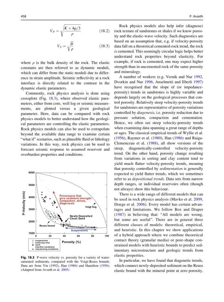
Commonly, rock physics analysis is done using
crossplots (Fig. 18.3), where observed elastic parameters, either from core, well log or seismic measurements, are plotted versus a given geological
parameter. Here, data can be compared with rock
physics models to better understand how the geological parameters are controlling the elastic parameters.
Rock physics models can also be used to extrapolate
beyond the available data range to examine certain
“what if” scenarios, such as plausible fluid or lithology
variations. In this way, rock physics can be used to
forecast seismic response to assumed reservoir and
overburden properties and conditions.
Rock physics models also help infer (diagnose)
rock texture of sandstones or shales if we know porosity and the elastic-wave velocity. Such diagnostics are
based on an assumption that, e.g. if velocity-porosity
data fall on a theoretical cemented-rock trend, the rock
is cemented. This seemingly circular logic helps better
understand rock properties beyond elasticity. For
example, if rock is cemented, one may expect higher
strength than in uncemented rock of the same porosity
and mineralogy.
A number of workers (e.g. Vernik and Nur 1992,
Dvorkin and Nur 1996, Anselmetti and Eberli 1997)
have recognised that the slope of (or impedanceporosity) trends in sandstones is highly variable and
depends largely on the geological processes that control porosity. Relatively steep velocity-porosity trends
for sandstones are representative of porosity variations
controlled by diagenesis, i.e. porosity reduction due to
pressure solution, compaction and cementation.
Hence, we often see steep velocity-porosity trends
when examining data spanning a great range of depths
or ages. The classical empirical trends of Wyllie et al.
(1956), Raymer et al. (1980), Han (1986) and RaigaClemenceau et al. (1988), all show versions of the
steep, diagenetically-controlled velocity-porosity
trend. On the other hand, porosity change resulting
from variations in sorting and clay content tend to
yield much flatter velocity-porosity trends, meaning
that porosity controlled by sedimentation is generally
expected to yield flatter trends, which we sometimes
refer to as depositional trends. Data sets from narrow
depth ranges, or individual reservoirs often (though
not always) show this behaviour.
There is a wide range of different models that can
be used in rock physics analysis (Mavko et al. 2009,
Dræge et al. 2006). Every model has certain advantages and limitations. We follow Box and Draper
(1987) in believing that: “All models are wrong,
but some are useful”. There are in general three
different classes of models: theoretical, empirical,
and heuristic. In this chapter we show applications
of a hybrid approach where we combine theoretical
contact theory (granular media) or pore-shape constrained models with heuristic bounds to predict sedimentary microstructure and geologic trends from
elastic properties.
In particular, we have found that diagenetic trends,
which connect newly-deposited sediment on the Reuss
elastic bound with the mineral point at zero porosity,
1000
2000
3000
4000
5000
6000
0
20
40
60
80
100
suspensions
sand-clay mixt.
sand
clay-free sandstone
clay-bearing sandstone
P-Velocity (m/s)
Porosity (%)
Voigt Avg.
Reuss bound
Suspensions
Newly Deposited
Clean Sand
Processess that
give sediment strength:
compaction, stress,
diagenesis
Fig. 18.3 P-wave velocity vs. porosity for a variety of watersaturated sediments, compared with the Voigt-Reuss bounds.
Data are from Yin (1992), Han (1986) and Hamilton (1956).
(Adapted from Avseth et al. 2005)
458
P. Avseth
ffiffiffiffiffiffiffiffiffiffiffiffiffiffiffiffiffiffiffi
K þ 4μ=3
ρ
s
ð18:2Þ
V S ¼
ffiffiffi
μ
ρ
r
ð18:3Þ
where ρ is the bulk density of the rock. The elastic
constants are then referred to as dynamic moduli,
which can differ from the static moduli due to difference in strain amplitude. Seismic reflectivity at a rock
interface is directly related to the contrast in the
dynamic elastic parameters.
Commonly, rock physics analysis is done using
crossplots (Fig. 18.3), where observed elastic parameters, either from core, well log or seismic measurements, are plotted versus a given geological
parameter. Here, data can be compared with rock
physics models to better understand how the geological parameters are controlling the elastic parameters.
Rock physics models can also be used to extrapolate
beyond the available data range to examine certain
“what if” scenarios, such as plausible fluid or lithology
variations. In this way, rock physics can be used to
forecast seismic response to assumed reservoir and
overburden properties and conditions.
Rock physics models also help infer (diagnose)
rock texture of sandstones or shales if we know porosity and the elastic-wave velocity. Such diagnostics are
based on an assumption that, e.g. if velocity-porosity
data fall on a theoretical cemented-rock trend, the rock
is cemented. This seemingly circular logic helps better
understand rock properties beyond elasticity. For
example, if rock is cemented, one may expect higher
strength than in uncemented rock of the same porosity
and mineralogy.
A number of workers (e.g. Vernik and Nur 1992,
Dvorkin and Nur 1996, Anselmetti and Eberli 1997)
have recognised that the slope of (or impedanceporosity) trends in sandstones is highly variable and
depends largely on the geological processes that control porosity. Relatively steep velocity-porosity trends
for sandstones are representative of porosity variations
controlled by diagenesis, i.e. porosity reduction due to
pressure solution, compaction and cementation.
Hence, we often see steep velocity-porosity trends
when examining data spanning a great range of depths
or ages. The classical empirical trends of Wyllie et al.
(1956), Raymer et al. (1980), Han (1986) and RaigaClemenceau et al. (1988), all show versions of the
steep, diagenetically-controlled velocity-porosity
trend. On the other hand, porosity change resulting
from variations in sorting and clay content tend to
yield much flatter velocity-porosity trends, meaning
that porosity controlled by sedimentation is generally
expected to yield flatter trends, which we sometimes
refer to as depositional trends. Data sets from narrow
depth ranges, or individual reservoirs often (though
not always) show this behaviour.
There is a wide range of different models that can
be used in rock physics analysis (Mavko et al. 2009,
Dræge et al. 2006). Every model has certain advantages and limitations. We follow Box and Draper
(1987) in believing that: “All models are wrong,
but some are useful”. There are in general three
different classes of models: theoretical, empirical,
and heuristic. In this chapter we show applications
of a hybrid approach where we combine theoretical
contact theory (granular media) or pore-shape constrained models with heuristic bounds to predict sedimentary microstructure and geologic trends from
elastic properties.
In particular, we have found that diagenetic trends,
which connect newly-deposited sediment on the Reuss
elastic bound with the mineral point at zero porosity,
1000
2000
3000
4000
5000
6000
0
20
40
60
80
100
suspensions
sand-clay mixt.
sand
clay-free sandstone
clay-bearing sandstone
P-Velocity (m/s)
Porosity (%)
Voigt Avg.
Reuss bound
Suspensions
Newly Deposited
Clean Sand
Processess that
give sediment strength:
compaction, stress,
diagenesis
Fig. 18.3 P-wave velocity vs. porosity for a variety of watersaturated sediments, compared with the Voigt-Reuss bounds.
Data are from Yin (1992), Han (1986) and Hamilton (1956).
(Adapted from Avseth et al. 2005)
458
P. Avseth