

to reduce smearing or inappropriate mixing of data
(Fig. 17.22). DMO is not routinely employed; however, it can be useful to solve the problem of
conflicting dip.
In practice, a velocity analysis has to be carried out,
where the main purpose is to determine the velocity
distribution as a function of time which will give the
most accurate NMO correction. The velocity analysis
is used to compute corrections in traveltime that will
be applied to all the traces belonging to a CMP-gather.
The most common type of velocity analysis is to
repeat the procedure of correcting and stacking CMP
data for many different velocities and within a discrete
time window. By measuring the average absolute
value of the data or more precisely the semblance
within time-windows of different test velocities, and
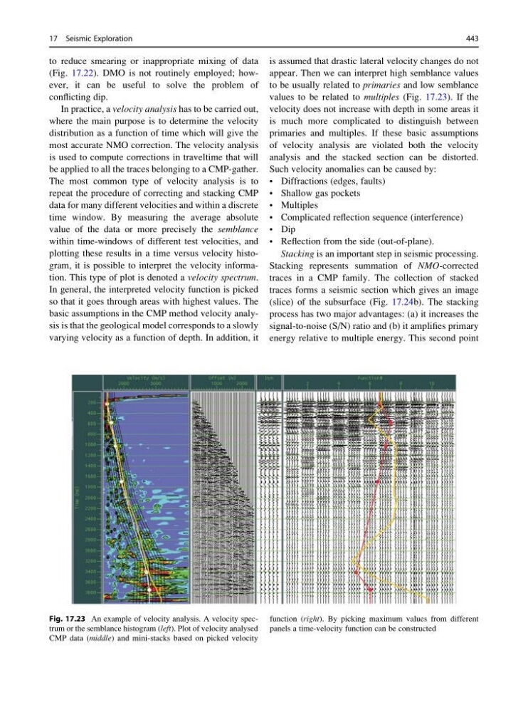
plotting these results in a time versus velocity histogram, it is possible to interpret the velocity information. This type of plot is denoted a velocity spectrum.
In general, the interpreted velocity function is picked
so that it goes through areas with highest values. The
basic assumptions in the CMP method velocity analysis is that the geological model corresponds to a slowly
varying velocity as a function of depth. In addition, it
is assumed that drastic lateral velocity changes do not
appear. Then we can interpret high semblance values
to be usually related to primaries and low semblance
values to be related to multiples (Fig. 17.23). If the
velocity does not increase with depth in some areas it
is much more complicated to distinguish between
primaries and multiples. If these basic assumptions
of velocity analysis are violated both the velocity
analysis and the stacked section can be distorted.
Such velocity anomalies can be caused by:
• Diffractions (edges, faults)
• Shallow gas pockets
• Multiples
• Complicated reflection sequence (interference)
• Dip
• Reflection from the side (out-of-plane).
Stacking is an important step in seismic processing.
Stacking represents summation of NMO-corrected
traces in a CMP family. The collection of stacked
traces forms a seismic section which gives an image
(slice) of the subsurface (Fig. 17.24b). The stacking
process has two major advantages: (a) it increases the
signal-to-noise (S/N) ratio and (b) it amplifies primary
energy relative to multiple energy. This second point
Fig. 17.23 An example of velocity analysis. A velocity spectrum or the semblance histogram (left). Plot of velocity analysed
CMP data (middle) and mini-stacks based on picked velocity
function (right). By picking maximum values from different
panels a time-velocity function can be constructed
17 Seismic Exploration
443
(Fig. 17.22). DMO is not routinely employed; however, it can be useful to solve the problem of
conflicting dip.
In practice, a velocity analysis has to be carried out,
where the main purpose is to determine the velocity
distribution as a function of time which will give the
most accurate NMO correction. The velocity analysis
is used to compute corrections in traveltime that will
be applied to all the traces belonging to a CMP-gather.
The most common type of velocity analysis is to
repeat the procedure of correcting and stacking CMP
data for many different velocities and within a discrete
time window. By measuring the average absolute
value of the data or more precisely the semblance
within time-windows of different test velocities, and
plotting these results in a time versus velocity histogram, it is possible to interpret the velocity information. This type of plot is denoted a velocity spectrum.
In general, the interpreted velocity function is picked
so that it goes through areas with highest values. The
basic assumptions in the CMP method velocity analysis is that the geological model corresponds to a slowly
varying velocity as a function of depth. In addition, it
is assumed that drastic lateral velocity changes do not
appear. Then we can interpret high semblance values
to be usually related to primaries and low semblance
values to be related to multiples (Fig. 17.23). If the
velocity does not increase with depth in some areas it
is much more complicated to distinguish between
primaries and multiples. If these basic assumptions
of velocity analysis are violated both the velocity
analysis and the stacked section can be distorted.
Such velocity anomalies can be caused by:
• Diffractions (edges, faults)
• Shallow gas pockets
• Multiples
• Complicated reflection sequence (interference)
• Dip
• Reflection from the side (out-of-plane).
Stacking is an important step in seismic processing.
Stacking represents summation of NMO-corrected
traces in a CMP family. The collection of stacked
traces forms a seismic section which gives an image
(slice) of the subsurface (Fig. 17.24b). The stacking
process has two major advantages: (a) it increases the
signal-to-noise (S/N) ratio and (b) it amplifies primary
energy relative to multiple energy. This second point
Fig. 17.23 An example of velocity analysis. A velocity spectrum or the semblance histogram (left). Plot of velocity analysed
CMP data (middle) and mini-stacks based on picked velocity
function (right). By picking maximum values from different
panels a time-velocity function can be constructed
17 Seismic Exploration
443