

Partie 3 – Probabilités
• Si X → U ([0 ; 1]), alors X pour densité f telle que
f (x) = 1 si x ∈ [0, 1] ; f (x) = 0 sinon
et pour fonction de répartition F X telle que
F X (x) =
0 si x 0
x si 0 x 1
1 si x 1
Une telle variable est simulée par la fonction « ÖÖÒÒÓÑ » du langage
PASCAL.
• Si X → U ([0 ; 1]), alors Y = a+(b − a) X → U ([a, b]) (a < b). Pour
établir ce résultat, on détermine F Y , f.r de Y . Pour tout x ∈ R :
F Y (x) = P (Y x) = P (a + (b − a) X x) = P
X
x − a
b − a
,
donc
F Y (x) = F X
x − a
b − a
=
⎧
⎪ ⎨
⎪ ⎩
0
six a
x − a
b − a
si a x b
1
six b
Car w : x →
x−a
b−a est une bijection strictement croissante de R sur
R, avec w (a) = 0 et w (b) = 1. On a bien Y → U ([a, b]).
Si X → U ([0 ; 1]), alors Y = a + (b − a) X → U ([a, b]) (a < b).
On utilise ce résultat pour simuler une v.a suivant la loi U ([a, b]).
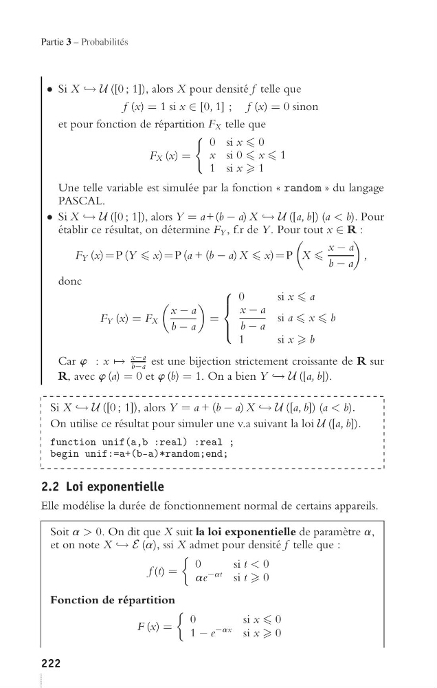
ÙÒÒØØÓÒ ÙÒÒÒ´´¸¸ ÖÖÖе ÖÖÖÐ
Ò ÙÒÒÒÒÒÒ·´´¹¹µ¶ÖÖÒÒÓÑÑÑÒÒÒ
2.2 Loi exponentielle
Elle modélise la durée de fonctionnement normal de certains appareils.
Soit a > 0. On dit que X suit la loi exponentielle de paramètre a,
et on note X → E (a), ssi X admet pour densité f telle que :
f (t) =
0
sit < 0
ae −at si t 0
Fonction de répartition
F (x) =
0
s ix 0
1 − e −ax si x 0
222
• Si X → U ([0 ; 1]), alors X pour densité f telle que
f (x) = 1 si x ∈ [0, 1] ; f (x) = 0 sinon
et pour fonction de répartition F X telle que
F X (x) =
0 si x 0
x si 0 x 1
1 si x 1
Une telle variable est simulée par la fonction « ÖÖÒÒÓÑ » du langage
PASCAL.
• Si X → U ([0 ; 1]), alors Y = a+(b − a) X → U ([a, b]) (a < b). Pour
établir ce résultat, on détermine F Y , f.r de Y . Pour tout x ∈ R :
F Y (x) = P (Y x) = P (a + (b − a) X x) = P
X
x − a
b − a
,
donc
F Y (x) = F X
x − a
b − a
=
⎧
⎪ ⎨
⎪ ⎩
0
six a
x − a
b − a
si a x b
1
six b
Car w : x →
x−a
b−a est une bijection strictement croissante de R sur
R, avec w (a) = 0 et w (b) = 1. On a bien Y → U ([a, b]).
Si X → U ([0 ; 1]), alors Y = a + (b − a) X → U ([a, b]) (a < b).
On utilise ce résultat pour simuler une v.a suivant la loi U ([a, b]).
ÙÒÒØØÓÒ ÙÒÒÒ´´¸¸ ÖÖÖе ÖÖÖÐ
Ò ÙÒÒÒÒÒÒ·´´¹¹µ¶ÖÖÒÒÓÑÑÑÒÒÒ
2.2 Loi exponentielle
Elle modélise la durée de fonctionnement normal de certains appareils.
Soit a > 0. On dit que X suit la loi exponentielle de paramètre a,
et on note X → E (a), ssi X admet pour densité f telle que :
f (t) =
0
sit < 0
ae −at si t 0
Fonction de répartition
F (x) =
0
s ix 0
1 − e −ax si x 0
222