

Estimation of Superpopulation Parameters
189
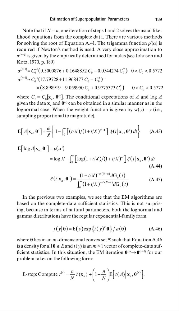
Note that if N 5 n, one iteration of steps 1 and 2 solves the usual likelihood equations from the complete data. There are various methods
for solving the root of Equation A.41. The trigamma function r'(a) is
required if Newton’s method is used. A very close approximation to
a
(v11) is given by the empirically determined formulas (see Johnson and
Kotz, 1970, p. 189)
( )
( )
1
1
2
0
0
0
0
1
1
2
1
0
0
0
2
0
0
0
0.5000876 0.1648852
0.0544274
0
0.5772
17.79728 11.968477
8.898919 9.059950
0.9775373
0
0.5772
(
)
(
)
(
)
v
v
C
C
C
C
C
C C
C
C
C
+
−
+
−
−
≈
+
−
<
<
≈
+
−
×
+
+
<
<
a
a
where C 0 5 C 0 [x n ,
(v)
]. The conditional expectations of A and log A
given the data x n and
(v) can be obtained in a similar manner as in the
lognormal case. When the weight function is given by w( y) 5 y (i.e.,
sampling proportional to magnitude),
' 1
0
'
E
, '
1
' 1
'
, '
'
( ) (
)
(
)
n
n
A
t
t
t
d t
∞
+
=
−
+
∫
x
x
a
a
l
l
j
l
(A.43)
'
0
E log
, '
'
log '
log 1
' 1
'
, '
( )
(
) (
)
(
)
n
n
A
t
t
t
d t
∞
=
=
−
+
+
∫
x
x
a
r a
l
l
l
j
(A.44)
(
)
(
)
'
'
0
1
'
G
, '
1
'
G
(
)
( )
(
)
(
)
( )
N n
n
n
N n
n
t
d
t
t
t
d
t
−
−
∞
−
−
+
=
+
∫
x
a
a
l
j
l
(A.45)
In the previous two examples, we see that the EM algorithms are
based on the complete-data suffi cient statistics. This is not surprising, because in terms of natural parameters, both the lognormal and
gamma distributions have the regular exponential-family form
{
}
b
exp
( ) ( )
( )
( )
T
f y
y
t y
a
=
(A.46)
where lies in an m -dimensional convex set Ξ such that Equation A.46
is a density for all ∊ E and t ( y) is an m × 1 vector of complete-data suffi cient statistics. In this situation, the EM iteration
(v)
→
(v11) for our
problem takes on the following form:
E-step: Compute
( )
( )
( ) 1
E ( ) ,
.
v
v
n
n
n
n
t
t
t A
N
N
=
+ −
x
x
189
Note that if N 5 n, one iteration of steps 1 and 2 solves the usual likelihood equations from the complete data. There are various methods
for solving the root of Equation A.41. The trigamma function r'(a) is
required if Newton’s method is used. A very close approximation to
a
(v11) is given by the empirically determined formulas (see Johnson and
Kotz, 1970, p. 189)
( )
( )
1
1
2
0
0
0
0
1
1
2
1
0
0
0
2
0
0
0
0.5000876 0.1648852
0.0544274
0
0.5772
17.79728 11.968477
8.898919 9.059950
0.9775373
0
0.5772
(
)
(
)
(
)
v
v
C
C
C
C
C
C C
C
C
C
+
−
+
−
−
≈
+
−
<
<
≈
+
−
×
+
+
<
<
a
a
where C 0 5 C 0 [x n ,
(v)
]. The conditional expectations of A and log A
given the data x n and
(v) can be obtained in a similar manner as in the
lognormal case. When the weight function is given by w( y) 5 y (i.e.,
sampling proportional to magnitude),
' 1
0
'
E
, '
1
' 1
'
, '
'
( ) (
)
(
)
n
n
A
t
t
t
d t
∞
+
=
−
+
∫
x
x
a
a
l
l
j
l
(A.43)
'
0
E log
, '
'
log '
log 1
' 1
'
, '
( )
(
) (
)
(
)
n
n
A
t
t
t
d t
∞
=
=
−
+
+
∫
x
x
a
r a
l
l
l
j
(A.44)
(
)
(
)
'
'
0
1
'
G
, '
1
'
G
(
)
( )
(
)
(
)
( )
N n
n
n
N n
n
t
d
t
t
t
d
t
−
−
∞
−
−
+
=
+
∫
x
a
a
l
j
l
(A.45)
In the previous two examples, we see that the EM algorithms are
based on the complete-data suffi cient statistics. This is not surprising, because in terms of natural parameters, both the lognormal and
gamma distributions have the regular exponential-family form
{
}
b
exp
( ) ( )
( )
( )
T
f y
y
t y
a
=
(A.46)
where lies in an m -dimensional convex set Ξ such that Equation A.46
is a density for all ∊ E and t ( y) is an m × 1 vector of complete-data suffi cient statistics. In this situation, the EM iteration
(v)
→
(v11) for our
problem takes on the following form:
E-step: Compute
( )
( )
( ) 1
E ( ) ,
.
v
v
n
n
n
n
t
t
t A
N
N
=
+ −
x
x