

188
Appendix A
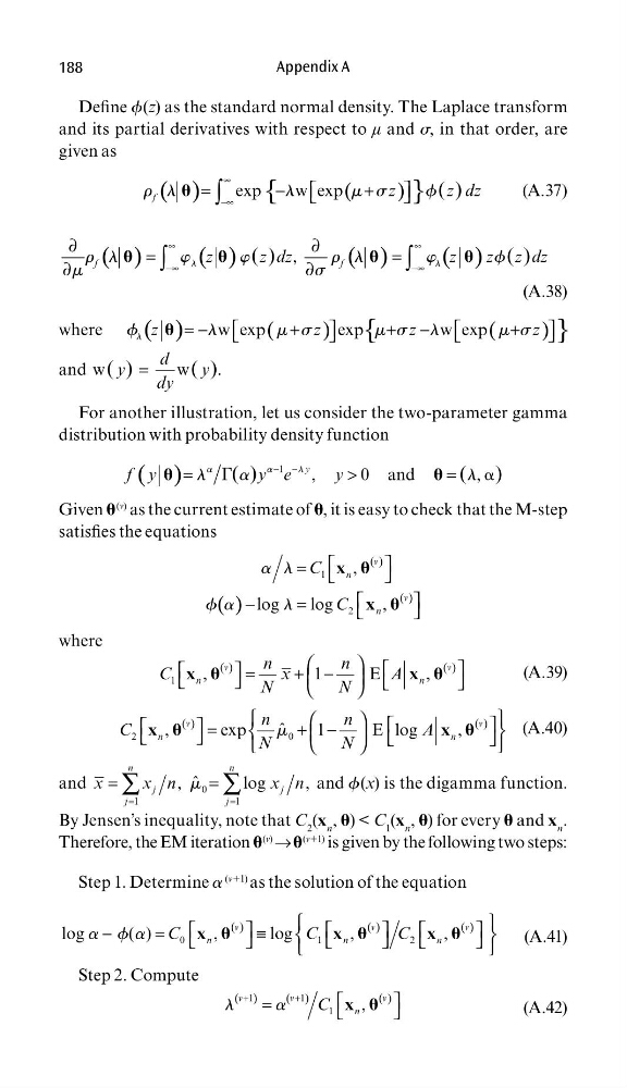
Defi ne f(z) as the standard normal density. The Laplace transform
and its partial derivatives with respect to μ and s, in that order, are
given as
( )
(
)
{
}
∞
−∞
=
−
+
∫ exp w exp
( )
f
z
z dz
r l
l
m s
f
(A.37)
( )
( )
( )
( )
∞
∞
−∞
−∞
∂
∂
=
=
∂
∂
∫
∫
,
( )
( )
f
f
z
z dz
z
z z dz
l
l
r l
w
w
r l
w
f
m
s
(A.38)
where
( )
(
)
(
)
{
}
= −
+
+ −
+
w exp
exp
w exp
z
z
z
z
l
f
l
m s
m s l
m s
and
=
w
w
.
( )
( )
d
y
y
dy
For another illustration, let us consider the two-parameter gamma
distribution with probability density function
( )
G
a
− −
=
>
=
1
,
0 and
,
( )
( )
y
f y
y e
y
a
a
l
l
a
l
Given
(v) as the current estimate of , it is easy to check that the M-step
satisfi es the equations
( )
( )
( )
=
−
=
1
2
,
log
log
,
v
n
v
n
C
C
x
x
a l
f a
l
where
( )
( )
=
+ −
1
,
1
E
,
v
v
n
n
n
n
C
x
A
N
N
x
x
(A.39)
( )
( )
=
+ −
2
0
ˆ
,
exp
1
E log
,
v
v
n
n
n
n
C
A
N
N
x
x
m
(A.40)
and
0
1
1
ˆ
,
l o g
,
n
n
j
j
j
j
x
x n
x n
=
=
=
=
∑
∑
m
and f(x) is the digamma function.
By Jensen’s inequality, note that C 2 (x n , ) < C 1 (x n , ) for every and x n .
Therefore, the EM iteration
(v)
→
(v11) is given by the following two steps:
Step 1. Determine a
(v11) as the solution of the equation
( )
( )
( )
0
1
2
log
( )
,
log
,
,
v
v
v
n
n
n
C
C
C
−
=
≡
x
x
x
a f a
(A.41)
Step 2. Compute
( )
( )
( )
1
1
1
,
v
v
v
n
C
+
+
=
x
l
a
(A.42)
Appendix A
Defi ne f(z) as the standard normal density. The Laplace transform
and its partial derivatives with respect to μ and s, in that order, are
given as
( )
(
)
{
}
∞
−∞
=
−
+
∫ exp w exp
( )
f
z
z dz
r l
l
m s
f
(A.37)
( )
( )
( )
( )
∞
∞
−∞
−∞
∂
∂
=
=
∂
∂
∫
∫
,
( )
( )
f
f
z
z dz
z
z z dz
l
l
r l
w
w
r l
w
f
m
s
(A.38)
where
( )
(
)
(
)
{
}
= −
+
+ −
+
w exp
exp
w exp
z
z
z
z
l
f
l
m s
m s l
m s
and
=
w
w
.
( )
( )
d
y
y
dy
For another illustration, let us consider the two-parameter gamma
distribution with probability density function
( )
G
a
− −
=
>
=
1
,
0 and
,
( )
( )
y
f y
y e
y
a
a
l
l
a
l
Given
(v) as the current estimate of , it is easy to check that the M-step
satisfi es the equations
( )
( )
( )
=
−
=
1
2
,
log
log
,
v
n
v
n
C
C
x
x
a l
f a
l
where
( )
( )
=
+ −
1
,
1
E
,
v
v
n
n
n
n
C
x
A
N
N
x
x
(A.39)
( )
( )
=
+ −
2
0
ˆ
,
exp
1
E log
,
v
v
n
n
n
n
C
A
N
N
x
x
m
(A.40)
and
0
1
1
ˆ
,
l o g
,
n
n
j
j
j
j
x
x n
x n
=
=
=
=
∑
∑
m
and f(x) is the digamma function.
By Jensen’s inequality, note that C 2 (x n , ) < C 1 (x n , ) for every and x n .
Therefore, the EM iteration
(v)
→
(v11) is given by the following two steps:
Step 1. Determine a
(v11) as the solution of the equation
( )
( )
( )
0
1
2
log
( )
,
log
,
,
v
v
v
n
n
n
C
C
C
−
=
≡
x
x
x
a f a
(A.41)
Step 2. Compute
( )
( )
( )
1
1
1
,
v
v
v
n
C
+
+
=
x
l
a
(A.42)