

Estimation of Superpopulation Parameters
185
given x n is the marginal distribution of A in (A, L), given the data. For a
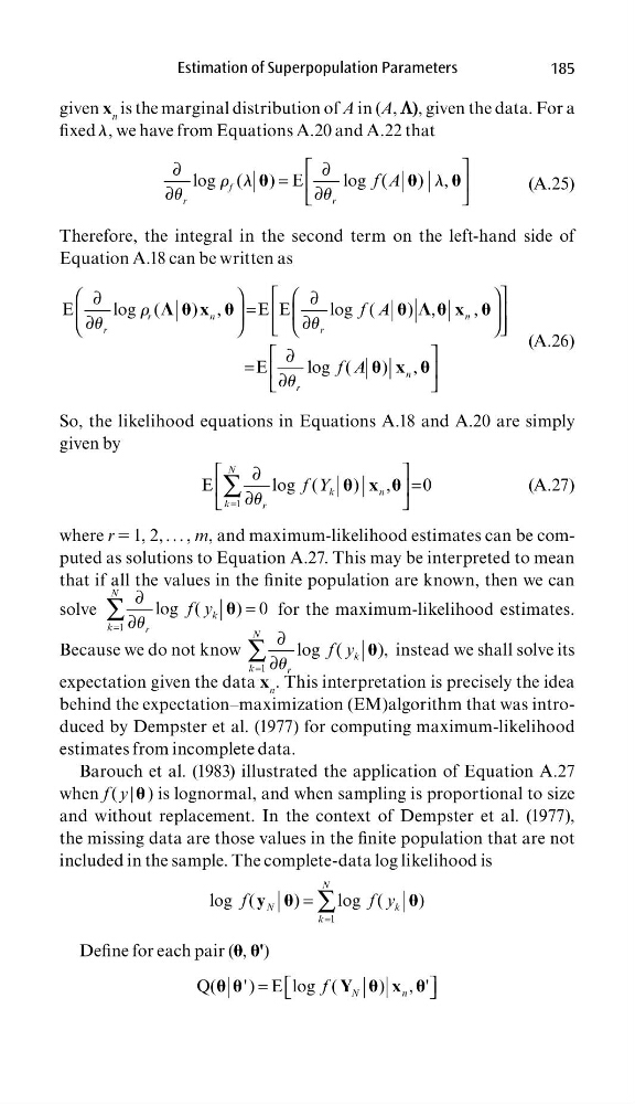
fi xed l, we have from Equations A.20 and A.22 that
log (
) E
log (
) ,
f
r
r
f A
∂
∂
=
∂
∂
r l
l
u
u
(A.25)
Therefore, the integral in the second term on the left-hand side of
Equation A.18 can be written as
E
log (
) ,
E E
log (
) ,
,
E
log (
) ,
r
n
n
r
r
n
r
f A
f A
⌳
⌳
∂
∂
=
∂
∂
∂
=
∂
x
x
x
r
u
u
u
(A.26)
So, the likelihood equations in Equations A.18 and A.20 are simply
given by
1
E
l o g (
)
,
0
N
k
n
k
r
f Y
=
∂
=
∂
∑
x
u
(A.27)
where r 5 1, 2, . . . , m, and maximum-likelihood estimates can be computed as solutions to Equation A.27. This may be interpreted to mean
that if all the values in the fi nite population are known, then we can
solve
1
log (
) 0
N
k
k
r
f y
=
∂
=
∂
∑ u
for the maximum-likelihood estimates.
Because we do not know
1
log (
),
N
k
k
r
f y
=
∂
∂
∑ u
instead we shall solve its
expectation given the data x n . This interpretation is precisely the idea
behind the expectation–maximization (EM)algorithm that was introduced by Dempster et al. (1977) for computing maximum-likelihood
estimates from incomplete data.
Barouch et al. (1983) illustrated the application of Equation A.27
when f ( y | ) is lognormal, and when sampling is proportional to size
and without replacement. In the context of Dempster et al. (1977),
the missing data are those values in the fi nite population that are not
included in the sample. The complete-data log likelihood is
1
log (
)
log (
)
N
N
k
k
f
fy
=
= ∑
y
Defi ne for each pair (, ')
Q(
' ) E log (
) , '
N
n
f
=
Y
x
185
given x n is the marginal distribution of A in (A, L), given the data. For a
fi xed l, we have from Equations A.20 and A.22 that
log (
) E
log (
) ,
f
r
r
f A
∂
∂
=
∂
∂
r l
l
u
u
(A.25)
Therefore, the integral in the second term on the left-hand side of
Equation A.18 can be written as
E
log (
) ,
E E
log (
) ,
,
E
log (
) ,
r
n
n
r
r
n
r
f A
f A
⌳
⌳
∂
∂
=
∂
∂
∂
=
∂
x
x
x
r
u
u
u
(A.26)
So, the likelihood equations in Equations A.18 and A.20 are simply
given by
1
E
l o g (
)
,
0
N
k
n
k
r
f Y
=
∂
=
∂
∑
x
u
(A.27)
where r 5 1, 2, . . . , m, and maximum-likelihood estimates can be computed as solutions to Equation A.27. This may be interpreted to mean
that if all the values in the fi nite population are known, then we can
solve
1
log (
) 0
N
k
k
r
f y
=
∂
=
∂
∑ u
for the maximum-likelihood estimates.
Because we do not know
1
log (
),
N
k
k
r
f y
=
∂
∂
∑ u
instead we shall solve its
expectation given the data x n . This interpretation is precisely the idea
behind the expectation–maximization (EM)algorithm that was introduced by Dempster et al. (1977) for computing maximum-likelihood
estimates from incomplete data.
Barouch et al. (1983) illustrated the application of Equation A.27
when f ( y | ) is lognormal, and when sampling is proportional to size
and without replacement. In the context of Dempster et al. (1977),
the missing data are those values in the fi nite population that are not
included in the sample. The complete-data log likelihood is
1
log (
)
log (
)
N
N
k
k
f
fy
=
= ∑
y
Defi ne for each pair (, ')
Q(
' ) E log (
) , '
N
n
f
=
Y
x