

184
Appendix A
provided the initial estimator u ˆ
n
(0) is suffi ciently close to u ˆ
n
, where U()
is the m × 1 vector of score functions defi ned by the left-hand side of
Equation A.18 and I 0 () is the second-derivative matrix of −log L().
This has (r, s) entry
2
0, ( )
log , 1 ,
rs
r
s
L
r s m
∂
= −
≤
≤
∂ ∂
I
u u
(A.21)
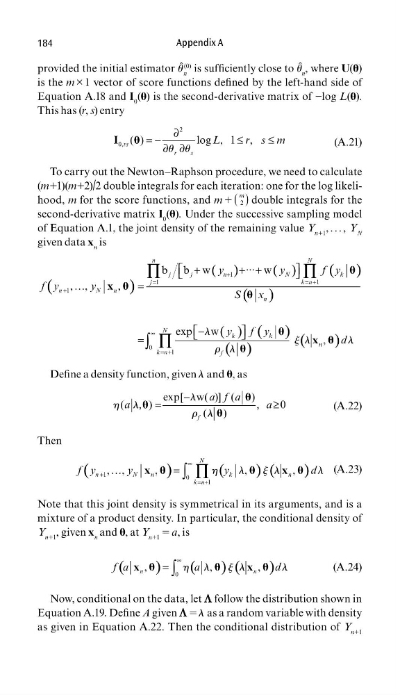
To carry out the Newton–Raphson procedure, we need to calculate
(m11)(m12) /2 double integrals for each iteration: one for the log likelihood, m for the score functions, and m 1 (
m
2 ) double integrals for the
second-derivative matrix I 0 (). Under the successive sampling model
of Equation A.1, the joint density of the remaining value Y n11 , . . . , Y N
given data x n is
(
)
( )
( )
( )
( )
( ) ( )
( )
(
)
+
=
= +
+
∞
= +
+
+ +
…
=
−
=
∏
∏
∏
∫
1
1
1
1
0
1
b b w
··· w
, ,
,
exp
w
,
n
N
j
j
n
N
k
j
k n
n
N
n
n
N
k
k
n
k n
f
y
y
f y
f y
y
S
x
y
f y
d
x
x
l
j l
l
r l
Defi ne a density function, given l and , as
−
=
≥
exp[ w( )] (
)
( , )
,
0
(
)
f
a f a
a
a
l
h l
r l
(A.22)
Then
(
)
(
) (
)
∞
+
= +
= ∏
∫
!
1
0
1
, ,
,
,
,
N
n
N
n
k
n
k n
f y
y
y
d
x
x
h
l
j l
l
(A.23)
Note that this joint density is symmetrical in its arguments, and is a
mixture of a product density. In particular, the conditional density of
Y n11 , given x n and , at Y n11 5 a, is
(
)
(
) (
)
∞
= ∫ 0
,
,
,
n
n
f a
a
d
x
x
h l
j l
l
(A.24)
Now, conditional on the data, let L follow the distribution shown in
Equation A.19. Defi ne A given L 5 l as a random variable with density
as given in Equation A.22. Then the conditional distribution of Y n11
Appendix A
provided the initial estimator u ˆ
n
(0) is suffi ciently close to u ˆ
n
, where U()
is the m × 1 vector of score functions defi ned by the left-hand side of
Equation A.18 and I 0 () is the second-derivative matrix of −log L().
This has (r, s) entry
2
0, ( )
log , 1 ,
rs
r
s
L
r s m
∂
= −
≤
≤
∂ ∂
I
u u
(A.21)
To carry out the Newton–Raphson procedure, we need to calculate
(m11)(m12) /2 double integrals for each iteration: one for the log likelihood, m for the score functions, and m 1 (
m
2 ) double integrals for the
second-derivative matrix I 0 (). Under the successive sampling model
of Equation A.1, the joint density of the remaining value Y n11 , . . . , Y N
given data x n is
(
)
( )
( )
( )
( )
( ) ( )
( )
(
)
+
=
= +
+
∞
= +
+
+ +
…
=
−
=
∏
∏
∏
∫
1
1
1
1
0
1
b b w
··· w
, ,
,
exp
w
,
n
N
j
j
n
N
k
j
k n
n
N
n
n
N
k
k
n
k n
f
y
y
f y
f y
y
S
x
y
f y
d
x
x
l
j l
l
r l
Defi ne a density function, given l and , as
−
=
≥
exp[ w( )] (
)
( , )
,
0
(
)
f
a f a
a
a
l
h l
r l
(A.22)
Then
(
)
(
) (
)
∞
+
= +
= ∏
∫
!
1
0
1
, ,
,
,
,
N
n
N
n
k
n
k n
f y
y
y
d
x
x
h
l
j l
l
(A.23)
Note that this joint density is symmetrical in its arguments, and is a
mixture of a product density. In particular, the conditional density of
Y n11 , given x n and , at Y n11 5 a, is
(
)
(
) (
)
∞
= ∫ 0
,
,
,
n
n
f a
a
d
x
x
h l
j l
l
(A.24)
Now, conditional on the data, let L follow the distribution shown in
Equation A.19. Defi ne A given L 5 l as a random variable with density
as given in Equation A.22. Then the conditional distribution of Y n11