

Estimation of Superpopulation Parameters
183
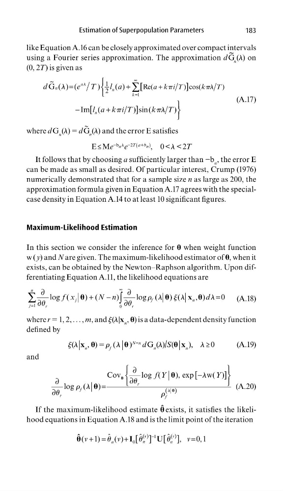
like Equation A.16 can be closely approximated over compact intervals
using a Fourier series approximation. The approximation d G
~
n
(l) on
(0, 2T) is given as
∞
=
+
=
+
−
+
∑
1
~
1
2
Re(
) cos(
)
G ( ) (
)
( )
Im (
) sin(
)
[
]
[
]
k
a
n
n
n
a k i T
k
T
d
e T
l a
l a k i T
k
T
l
p
p l
l
p
p l
(A.17)
where d G n (l) 5 d G
~
n
(l) and the error E satisfi es
E ≤ Me
−b n l e
−2T ( a1b n ) , 0 < l < 2T
It follows that by choosing a suffi ciently larger than −b n , the error E
can be made as small as desired. Of particular interest, Crump (1976)
numerically demonstrated that for a sample size n as large as 200, the
approximation formula given in Equation A.17 agrees with the specialcase density in Equation A.14 to at least 10 signifi cant fi gures.
Maximum-Likelihood Estimation
In this section we consider the inference for when weight function
w ( y) and N are given. The maximum-likelihood estimator of , when it
exists, can be obtained by the Newton–Raphson algorithm. Upon differentiating Equation A.11, the likelihood equations are
1
0
log (
) (
)
log (
) (
, )
0
n
j
f
n
j
r
r
f x
N n
d
∞
=
∂
∂
+
−
=
∂
∂
∑
∫
x
r l j l
l
u
u
(A.18)
where r 5 1, 2, . . . , m, and j(l|x n , ) is a data-dependent density function
defi ned by
j (l | x n , ) 5 r f ( l | )
N−n d G n (l)/S( | x n ), l ≥ 0
(A.19)
and
( )
∂
−
∂
∂
=
∂
Cov
log (
), exp
w( )
log (
)
[
]
r
f
r
f
f Y
Y
l
l
u
r l
u
r
(A.20)
If the maximum-likelihood estimate ˆ exists, it satisfi es the likelihood equations in Equation A.18 and is the limit point of the iteration
( )
( )
−
+ =
+
=
1
0
ˆ
ˆ
ˆ
( 1)
( )
,
0,1
[ ] [ ]
v
v
n
n
n
v
v
v
ˆ
I
U
u
u
u
183
like Equation A.16 can be closely approximated over compact intervals
using a Fourier series approximation. The approximation d G
~
n
(l) on
(0, 2T) is given as
∞
=
+
=
+
−
+
∑
1
~
1
2
Re(
) cos(
)
G ( ) (
)
( )
Im (
) sin(
)
[
]
[
]
k
a
n
n
n
a k i T
k
T
d
e T
l a
l a k i T
k
T
l
p
p l
l
p
p l
(A.17)
where d G n (l) 5 d G
~
n
(l) and the error E satisfi es
E ≤ Me
−b n l e
−2T ( a1b n ) , 0 < l < 2T
It follows that by choosing a suffi ciently larger than −b n , the error E
can be made as small as desired. Of particular interest, Crump (1976)
numerically demonstrated that for a sample size n as large as 200, the
approximation formula given in Equation A.17 agrees with the specialcase density in Equation A.14 to at least 10 signifi cant fi gures.
Maximum-Likelihood Estimation
In this section we consider the inference for when weight function
w ( y) and N are given. The maximum-likelihood estimator of , when it
exists, can be obtained by the Newton–Raphson algorithm. Upon differentiating Equation A.11, the likelihood equations are
1
0
log (
) (
)
log (
) (
, )
0
n
j
f
n
j
r
r
f x
N n
d
∞
=
∂
∂
+
−
=
∂
∂
∑
∫
x
r l j l
l
u
u
(A.18)
where r 5 1, 2, . . . , m, and j(l|x n , ) is a data-dependent density function
defi ned by
j (l | x n , ) 5 r f ( l | )
N−n d G n (l)/S( | x n ), l ≥ 0
(A.19)
and
( )
∂
−
∂
∂
=
∂
Cov
log (
), exp
w( )
log (
)
[
]
r
f
r
f
f Y
Y
l
l
u
r l
u
r
(A.20)
If the maximum-likelihood estimate ˆ exists, it satisfi es the likelihood equations in Equation A.18 and is the limit point of the iteration
( )
( )
−
+ =
+
=
1
0
ˆ
ˆ
ˆ
( 1)
( )
,
0,1
[ ] [ ]
v
v
n
n
n
v
v
v
ˆ
I
U
u
u
u