

182
Appendix A
1
( 1)
n l
l
i l
n i
C
l i
−
≠
− +
= −
−
∏
so that
−
−
−
= −
1
b
( 1)
1
n l
l
l
n
C
n
l
(A.13)
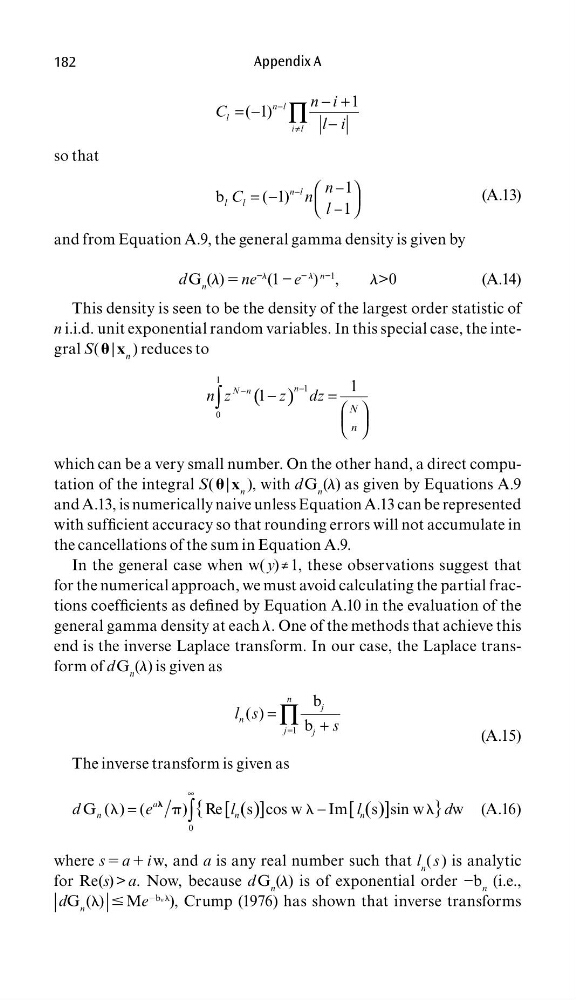
and from Equation A.9, the general gamma density is given by
d G n (l) 5 ne
−l (1 − e
− l
)
n−1
,
l>0
(A.14)
This density is seen to be the density of the largest order statistic of
n i.i.d. unit exponential random variables. In this special case, the integral S( | x n ) reduces to
( )
−
−
−
=
∫
1
1
0
1
1
n
N n
N
n
n z
z dz
which can be a very small number. On the other hand, a direct computation of the integral S( | x n ), with d G n (l) as given by Equations A.9
and A.13, is numerically naive unless Equation A.13 can be represented
with suffi cient accuracy so that rounding errors will not accumulate in
the cancellations of the sum in Equation A.9.
In the general case when w( y) ≠ 1, these observations suggest that
for the numerical approach, we must avoid calculating the partial fractions coeffi cients as defi ned by Equation A.10 in the evaluation of the
general gamma density at each l. One of the methods that achieve this
end is the inverse Laplace transform. In our case, the Laplace transform of d G n (l) is given as
1
b
( )
b
n
j
n
j
j
l s
s
=
=
+
∏
(A.15)
The inverse transform is given as
l
p
l
l
∞
=
−
∫
0
G ( ) (
) Re
s cos w
Im
s sin w
w
[
]
[
]
( )
( )
{
}
a
n
n
n
d
e
l
l
d
(A.16)
where s 5 a 1 i w, and a is any real number such that l n ( s ) is analytic
for Re(s) > a. Now, because d G n (l) is of exponential order −b n (i.e.,
| dG n (l) | # Me
2bn l
), Crump (1976) has shown that inverse transforms
Appendix A
1
( 1)
n l
l
i l
n i
C
l i
−
≠
− +
= −
−
∏
so that
−
−
−
= −
1
b
( 1)
1
n l
l
l
n
C
n
l
(A.13)
and from Equation A.9, the general gamma density is given by
d G n (l) 5 ne
−l (1 − e
− l
)
n−1
,
l>0
(A.14)
This density is seen to be the density of the largest order statistic of
n i.i.d. unit exponential random variables. In this special case, the integral S( | x n ) reduces to
( )
−
−
−
=
∫
1
1
0
1
1
n
N n
N
n
n z
z dz
which can be a very small number. On the other hand, a direct computation of the integral S( | x n ), with d G n (l) as given by Equations A.9
and A.13, is numerically naive unless Equation A.13 can be represented
with suffi cient accuracy so that rounding errors will not accumulate in
the cancellations of the sum in Equation A.9.
In the general case when w( y) ≠ 1, these observations suggest that
for the numerical approach, we must avoid calculating the partial fractions coeffi cients as defi ned by Equation A.10 in the evaluation of the
general gamma density at each l. One of the methods that achieve this
end is the inverse Laplace transform. In our case, the Laplace transform of d G n (l) is given as
1
b
( )
b
n
j
n
j
j
l s
s
=
=
+
∏
(A.15)
The inverse transform is given as
l
p
l
l
∞
=
−
∫
0
G ( ) (
) Re
s cos w
Im
s sin w
w
[
]
[
]
( )
( )
{
}
a
n
n
n
d
e
l
l
d
(A.16)
where s 5 a 1 i w, and a is any real number such that l n ( s ) is analytic
for Re(s) > a. Now, because d G n (l) is of exponential order −b n (i.e.,
| dG n (l) | # Me
2bn l
), Crump (1976) has shown that inverse transforms