

Estimation of Superpopulation Parameters
181
In general, the integral S(|x n ) does not have a closed form for most
of the commonly used superpopulation distributions, such as the lognormal distribution. Barouch and Kaufman (1977) computed a uniform asymptotic expansion for the density given in Equation A.8 when
f u is lognormal, 5 (μ, s), and w( y) 5 y, then used it to approximate a
likelihood function for μ, s, and N given the data x n . Approximate conditional maximum-likelihood estimators for μ and s
2 , given N, were
shown to be the unique maximizer of the uniform approximation to the
likelihood. Although the uniform asymptotic approximation is valid
for a wide range of possible parameter values of the lognormal density
and for large N − n, its practical usage is somewhat limited. Estimates
for the standard errors of the approximate conditional maximum-likelihood estimators are also not readily available.
Alternatively, the log-likelihood function of Equation A.11 may be
numerically evaluated for each , given the observed data x n . At a casual
glance at the integral in Equation A.12 with d G n (l) given by Equations
A.9 and A.10, it appears that the most diffi cult part is the numerical
evaluation of r f ( l|) coupled with a suitable numerical quadrature
routine. A closer examination (Barouch and Kaufman, 1977) reveals
that the problem lies in the accurate evaluation of the general gamma
density when l is small. A direct calculation based on the density as
defi ned by Equations A.9 and A.10 turns out to be numerically unfeasible unless the sample size n is small.
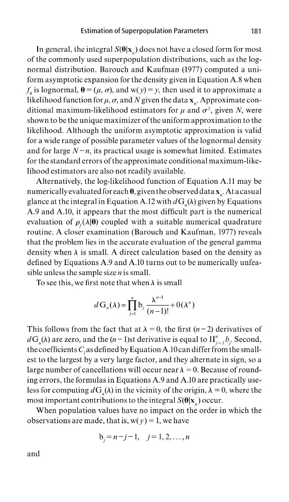
To see this, we fi rst note that when l is small
l
−
=
=
+
−
∏
1
1
G ( )
b
0( )
( 1)!
n
n
n
n
j
j
d
n
l
l
This follows from the fact that at l 5 0, the fi rst (n − 2) derivatives of
d G n (l) are zero, and the (n − 1)st derivative is equal to P
n
j 5 1
b j . Second,
the coeffi cients C l as defi ned by Equation A.10 can differ from the smallest to the largest by a very large factor, and they alternate in sign, so a
large number of cancellations will occur near l 5 0. Because of rounding errors, the formulas in Equations A.9 and A.10 are practically useless for computing d G n (l) in the vicinity of the origin, l 5 0, where the
most important contributions to the integral S(|x n ) occur.
When population values have no impact on the order in which the
observations are made, that is, w( y ) 5 1, we have
b j 5 n − j − 1, j 5 1, 2, . . . , n
and
181
In general, the integral S(|x n ) does not have a closed form for most
of the commonly used superpopulation distributions, such as the lognormal distribution. Barouch and Kaufman (1977) computed a uniform asymptotic expansion for the density given in Equation A.8 when
f u is lognormal, 5 (μ, s), and w( y) 5 y, then used it to approximate a
likelihood function for μ, s, and N given the data x n . Approximate conditional maximum-likelihood estimators for μ and s
2 , given N, were
shown to be the unique maximizer of the uniform approximation to the
likelihood. Although the uniform asymptotic approximation is valid
for a wide range of possible parameter values of the lognormal density
and for large N − n, its practical usage is somewhat limited. Estimates
for the standard errors of the approximate conditional maximum-likelihood estimators are also not readily available.
Alternatively, the log-likelihood function of Equation A.11 may be
numerically evaluated for each , given the observed data x n . At a casual
glance at the integral in Equation A.12 with d G n (l) given by Equations
A.9 and A.10, it appears that the most diffi cult part is the numerical
evaluation of r f ( l|) coupled with a suitable numerical quadrature
routine. A closer examination (Barouch and Kaufman, 1977) reveals
that the problem lies in the accurate evaluation of the general gamma
density when l is small. A direct calculation based on the density as
defi ned by Equations A.9 and A.10 turns out to be numerically unfeasible unless the sample size n is small.
To see this, we fi rst note that when l is small
l
−
=
=
+
−
∏
1
1
G ( )
b
0( )
( 1)!
n
n
n
n
j
j
d
n
l
l
This follows from the fact that at l 5 0, the fi rst (n − 2) derivatives of
d G n (l) are zero, and the (n − 1)st derivative is equal to P
n
j 5 1
b j . Second,
the coeffi cients C l as defi ned by Equation A.10 can differ from the smallest to the largest by a very large factor, and they alternate in sign, so a
large number of cancellations will occur near l 5 0. Because of rounding errors, the formulas in Equations A.9 and A.10 are practically useless for computing d G n (l) in the vicinity of the origin, l 5 0, where the
most important contributions to the integral S(|x n ) occur.
When population values have no impact on the order in which the
observations are made, that is, w( y ) 5 1, we have
b j 5 n − j − 1, j 5 1, 2, . . . , n
and