

186
Appendix A
Then the EM iteration
(v)
→
(v11) is defi ned as follows:
E-step: Compute Q [ |
(v)
].
M-step: Choose
(v11) to be a value of ∊ E, which maximizes
Q [ |
(v)
].
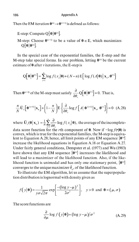
In the special case of the exponential families, the E-step and the
M-step take special forms. In our problem, letting
(v) be the current
estimate of after v iterations, the E-step is
( )
( )
=
=
+
−
∑
1
Q
log (
) (
) E log (
)
,
n
v
v
j
n
j
f x
N n
f A
x
Then
(v11) of the M-step must satisfy
( )
∂
=
∂
Q
0 .
v
r
u
That is,
( )
( )
( )
+
+
∂
+ −
=
∂
1
1
,
1
E
log
0
v
n
v
v
r
n
r
n
n
f A
N
N
U
x
x
u
(A.28)
where
1
1
(
)
log (
),
n
r
n
j
j
r
n
f x
=
∂
=
∂
∑
U
x
u
the average of the incompletedata score function for the rth component of . Now if −log f (•|) is
convex, which is true for the exponential families, the M-step is equivalent to Equation A.28; hence, all limit points of any EM sequence {
(v)
}
increase the likelihood equations in Equation A.18 or Equation A.27.
Under fairly general conditions, Dempster et al. (1977) and Wu (1983)
have shown that any EM sequence {
(v)
} increases the likelihood and
will lead to a maximizer of the likelihood function. Also, if the likelihood function is unimodal and has only one stationary point, {
(v)
}
converges to the unique maximizer u ˆ
n
, of the likelihood function.
To illustrate the EM algorithm, let us assume that the superpopulation distribution is lognormal with density given as
( )
(
)
(
)
−
−
=
>
=
2
2
log
1
exp
,
0 and
,
2
2
y
f y
y
y
m
m s
s
s p
The score functions are
( ) (
)
∂
=
−
∂
2
log
log
f y
y m s
m
(A.29)
Appendix A
Then the EM iteration
(v)
→
(v11) is defi ned as follows:
E-step: Compute Q [ |
(v)
].
M-step: Choose
(v11) to be a value of ∊ E, which maximizes
Q [ |
(v)
].
In the special case of the exponential families, the E-step and the
M-step take special forms. In our problem, letting
(v) be the current
estimate of after v iterations, the E-step is
( )
( )
=
=
+
−
∑
1
Q
log (
) (
) E log (
)
,
n
v
v
j
n
j
f x
N n
f A
x
Then
(v11) of the M-step must satisfy
( )
∂
=
∂
Q
0 .
v
r
u
That is,
( )
( )
( )
+
+
∂
+ −
=
∂
1
1
,
1
E
log
0
v
n
v
v
r
n
r
n
n
f A
N
N
U
x
x
u
(A.28)
where
1
1
(
)
log (
),
n
r
n
j
j
r
n
f x
=
∂
=
∂
∑
U
x
u
the average of the incompletedata score function for the rth component of . Now if −log f (•|) is
convex, which is true for the exponential families, the M-step is equivalent to Equation A.28; hence, all limit points of any EM sequence {
(v)
}
increase the likelihood equations in Equation A.18 or Equation A.27.
Under fairly general conditions, Dempster et al. (1977) and Wu (1983)
have shown that any EM sequence {
(v)
} increases the likelihood and
will lead to a maximizer of the likelihood function. Also, if the likelihood function is unimodal and has only one stationary point, {
(v)
}
converges to the unique maximizer u ˆ
n
, of the likelihood function.
To illustrate the EM algorithm, let us assume that the superpopulation distribution is lognormal with density given as
( )
(
)
(
)
−
−
=
>
=
2
2
log
1
exp
,
0 and
,
2
2
y
f y
y
y
m
m s
s
s p
The score functions are
( ) (
)
∂
=
−
∂
2
log
log
f y
y m s
m
(A.29)