

radiation. The mechanical implementation of these schemes, including elliptical
undulators, helical undulators, crossed undulators, and more exotic solutions, was
described in Chap. 2 [80].
One of the most flexible insertion devices for providing variable polarization is
the elliptical undulator, also called an elliptically polarizing undulator (‘EPU’). It
has a pair of perpendicular sinusoidal magnetic fields, which have the same periodicity but arbitrary relative phases and amplitudes, leading to a net on-axis magnetic
field b
B s
ð Þ (Eq. 3.57):
B
!
s
ð Þ ¼ b
B x0 sin
2π s
λ u
À ϕ
þ b
B y0 sin
2π s
λ u
ð3:57Þ
Since the elliptical undulator has two field components, it will have two K-values,
with the horizontal K x controlled by the strength of the vertical field and the vertical
K y controlled by the strength of the horizontal field (Fig. 3.18):
K x ¼ 0:934 b
B y0 T
½ λ u cm
½ K y ¼ 0:934 b
B x0 T
½ λ u cm
½
ð3:58Þ
3.8.1 Elliptical Undulator Power
The equation for total power is a slight modification of that for a planar undulator,
taking into account the two different fields.
P e‐und kW
½ ¼ 0:633E
2
e GeV
½
b
B
2
x0 þ b
B
2
y0
T
½ I A
½ L m
ð Þ
ð3:59Þ
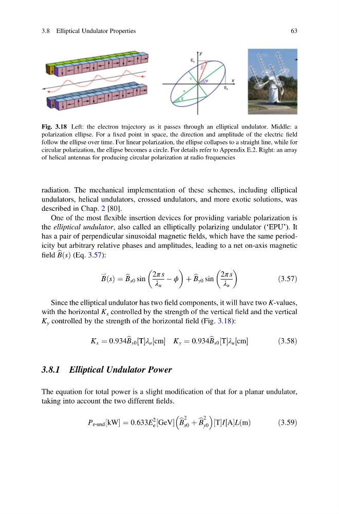
Fig. 3.18 Left: the electron trajectory as it passes through an elliptical undulator. Middle: a
polarization ellipse. For a fixed point in space, the direction and amplitude of the electric field
follow the ellipse over time. For linear polarization, the ellipse collapses to a straight line, while for
circular polarization, the ellipse becomes a circle. For details refer to Appendix E.2. Right: an array
of helical antennas for producing circular polarization at radio frequencies
3.8 Elliptical Undulator Properties
63
undulators, helical undulators, crossed undulators, and more exotic solutions, was
described in Chap. 2 [80].
One of the most flexible insertion devices for providing variable polarization is
the elliptical undulator, also called an elliptically polarizing undulator (‘EPU’). It
has a pair of perpendicular sinusoidal magnetic fields, which have the same periodicity but arbitrary relative phases and amplitudes, leading to a net on-axis magnetic
field b
B s
ð Þ (Eq. 3.57):
B
!
s
ð Þ ¼ b
B x0 sin
2π s
λ u
À ϕ
þ b
B y0 sin
2π s
λ u
ð3:57Þ
Since the elliptical undulator has two field components, it will have two K-values,
with the horizontal K x controlled by the strength of the vertical field and the vertical
K y controlled by the strength of the horizontal field (Fig. 3.18):
K x ¼ 0:934 b
B y0 T
½ λ u cm
½ K y ¼ 0:934 b
B x0 T
½ λ u cm
½
ð3:58Þ
3.8.1 Elliptical Undulator Power
The equation for total power is a slight modification of that for a planar undulator,
taking into account the two different fields.
P e‐und kW
½ ¼ 0:633E
2
e GeV
½
b
B
2
x0 þ b
B
2
y0
T
½ I A
½ L m
ð Þ
ð3:59Þ
Fig. 3.18 Left: the electron trajectory as it passes through an elliptical undulator. Middle: a
polarization ellipse. For a fixed point in space, the direction and amplitude of the electric field
follow the ellipse over time. For linear polarization, the ellipse collapses to a straight line, while for
circular polarization, the ellipse becomes a circle. For details refer to Appendix E.2. Right: an array
of helical antennas for producing circular polarization at radio frequencies
3.8 Elliptical Undulator Properties
63