

hν ¼ E
vacuum
binding þ E´ kinetic ¼ E
Fermi
binding þ φ spectrometer þ E kinetic þ . . .
ð11:1Þ
where E
vacuum
binding is the binding energy relative to the vacuum level, E´ kinetic is the
kinetic energy of the photoelectron as it leaves the sample, E
Fermi
binding is the binding
energy relative to the Fermi level, E kinetic is the kinetic energy as measured in the
spectrometer, and φ spectrometer is the work function of the spectrometer [509]. In
some cases, there are complications due to sample charging, and an additional
potential V charge needs to be added.
Photoelectron spectroscopy has a long history. Heinrich Hertz demonstrated
that light could cause an electrical current to flow from a sample in 1877 [510],
and in 1905 Einstein’s explanation of the photoelectric effect was a key step
toward quantum theory [511], and it led to his 1921 Nobel Prize, “for his
discovery of the law of the photoelectric effect” (although his Nobel lecture
was about relativity). In the mid-1950s, Kai Siegbahn built electron energy
analyzers with a precision of 10
À5
–10
À6 , and in multiple papers, he showed
that resolvable chemical shifts occur for atoms in different environments
(Fig. 11.2), leading to the acronym “ESCA”—“Electron Spectroscopy for Chemical Analysis” [512, 513]. Siegbahn received his own Nobel prize in physics in
1981, “for his contribution to the development of high-resolution electron spectroscopy [514].”
The first synchrotron XPS experiments were done by Pianetta and Lindau in
1974 at SSRL. They were forced to use hard X-rays because the beamline was cut
off from ring vacuum by Be windows. With 8 keV radiation, they observed the 4f
spin-orbit splitting for Au metal with ~0.35 eV instrumental resolution
(Fig. 11.4) [517].
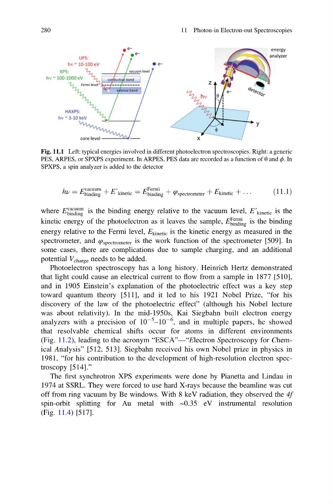
Fig. 11.1 Left: typical energies involved in different photoelectron spectroscopies. Right: a generic
PES, ARPES, or SPXPS experiment. In ARPES, PES data are recorded as a function of θ and ϕ. In
SPXPS, a spin analyzer is added to the detector
280
11 Photon-in Electron-out Spectroscopies
vacuum
binding þ E´ kinetic ¼ E
Fermi
binding þ φ spectrometer þ E kinetic þ . . .
ð11:1Þ
where E
vacuum
binding is the binding energy relative to the vacuum level, E´ kinetic is the
kinetic energy of the photoelectron as it leaves the sample, E
Fermi
binding is the binding
energy relative to the Fermi level, E kinetic is the kinetic energy as measured in the
spectrometer, and φ spectrometer is the work function of the spectrometer [509]. In
some cases, there are complications due to sample charging, and an additional
potential V charge needs to be added.
Photoelectron spectroscopy has a long history. Heinrich Hertz demonstrated
that light could cause an electrical current to flow from a sample in 1877 [510],
and in 1905 Einstein’s explanation of the photoelectric effect was a key step
toward quantum theory [511], and it led to his 1921 Nobel Prize, “for his
discovery of the law of the photoelectric effect” (although his Nobel lecture
was about relativity). In the mid-1950s, Kai Siegbahn built electron energy
analyzers with a precision of 10
À5
–10
À6 , and in multiple papers, he showed
that resolvable chemical shifts occur for atoms in different environments
(Fig. 11.2), leading to the acronym “ESCA”—“Electron Spectroscopy for Chemical Analysis” [512, 513]. Siegbahn received his own Nobel prize in physics in
1981, “for his contribution to the development of high-resolution electron spectroscopy [514].”
The first synchrotron XPS experiments were done by Pianetta and Lindau in
1974 at SSRL. They were forced to use hard X-rays because the beamline was cut
off from ring vacuum by Be windows. With 8 keV radiation, they observed the 4f
spin-orbit splitting for Au metal with ~0.35 eV instrumental resolution
(Fig. 11.4) [517].
Fig. 11.1 Left: typical energies involved in different photoelectron spectroscopies. Right: a generic
PES, ARPES, or SPXPS experiment. In ARPES, PES data are recorded as a function of θ and ϕ. In
SPXPS, a spin analyzer is added to the detector
280
11 Photon-in Electron-out Spectroscopies