

9.5.3 Quantum Beats 1: Quadrupole Splittings and Isomer
Shifts
For most experiments, it is the chemical properties of the Mössbauer nucleus that are
most of interest. For the remainder of the discussion, we assume a thin sample with
moderate dynamical beats. If the sample under consideration contains two resonance
lines, say from quadrupole splitting, then the interaction between those two frequencies is observed as “quantum beats.” If the separation Δω is large compared to their
effective linewidth, the resulting time spectrum can be approximated as the product
of the dynamical beat pattern and a quantum beat pattern reflecting the interference
between the two frequencies:
I τ
ð Þ / e
Àτ χ
τ
J
2
1
ffiffiffiffi ffi
χτ
τ
r
cos
2 Δω
2
t þ
χΓ 0
8ΔE
ð9:19Þ
A nice example of such quantum beats involves the NFS from ferrocene
(Fig. 9.14). The observed beat period of 35.8 ns yields a quadrupole splitting of
2.39 mm s
À1
.
Another chemically useful quantity that can be obtained from NFS is the isomer
shift. The absolute measurement of the γ-ray frequency with sufficient precision to
define shifts is obviously impossible, but the relative frequency and energy can be
obtained by observing beats between signals from the sample and a single-line
reference material [447]. As illustrated in Fig. 9.14, if one places a single-line
reference material in the beam before or after the sample, then there will be
interference between the forward scattering from this reference and from the sample.
The difference in isomer shifts can then be directly extracted from the beat frequency
in the forward scattering signal. For our ferrocene example, introduction of a
stainless steel reference introduced an extra beat in the NFS that was used to
calculate an isomer shift of 0.44 mm s
À1 (Fig. 9.14).
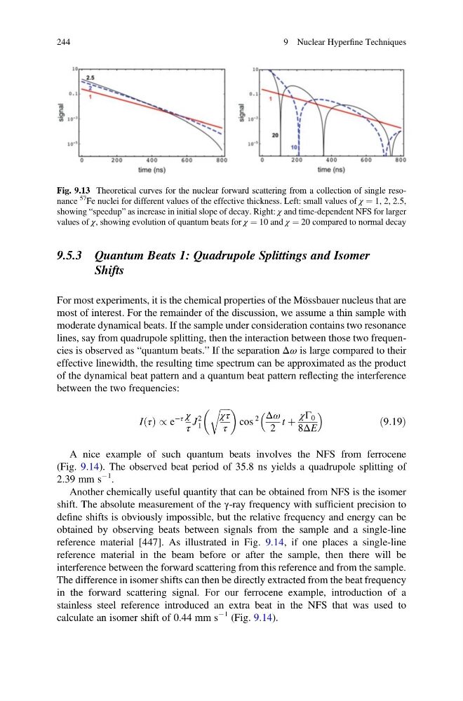
Fig. 9.13 Theoretical curves for the nuclear forward scattering from a collection of single resonance
57
Fe nuclei for different values of the effective thickness. Left: small values of χ ¼ 1, 2, 2.5,
showing “speedup” as increase in initial slope of decay. Right: χ and time-dependent NFS for larger
values of χ, showing evolution of quantum beats for χ ¼ 10 and χ ¼ 20 compared to normal decay
244
9 Nuclear Hyperfine Techniques
Shifts
For most experiments, it is the chemical properties of the Mössbauer nucleus that are
most of interest. For the remainder of the discussion, we assume a thin sample with
moderate dynamical beats. If the sample under consideration contains two resonance
lines, say from quadrupole splitting, then the interaction between those two frequencies is observed as “quantum beats.” If the separation Δω is large compared to their
effective linewidth, the resulting time spectrum can be approximated as the product
of the dynamical beat pattern and a quantum beat pattern reflecting the interference
between the two frequencies:
I τ
ð Þ / e
Àτ χ
τ
J
2
1
ffiffiffiffi ffi
χτ
τ
r
cos
2 Δω
2
t þ
χΓ 0
8ΔE
ð9:19Þ
A nice example of such quantum beats involves the NFS from ferrocene
(Fig. 9.14). The observed beat period of 35.8 ns yields a quadrupole splitting of
2.39 mm s
À1
.
Another chemically useful quantity that can be obtained from NFS is the isomer
shift. The absolute measurement of the γ-ray frequency with sufficient precision to
define shifts is obviously impossible, but the relative frequency and energy can be
obtained by observing beats between signals from the sample and a single-line
reference material [447]. As illustrated in Fig. 9.14, if one places a single-line
reference material in the beam before or after the sample, then there will be
interference between the forward scattering from this reference and from the sample.
The difference in isomer shifts can then be directly extracted from the beat frequency
in the forward scattering signal. For our ferrocene example, introduction of a
stainless steel reference introduced an extra beat in the NFS that was used to
calculate an isomer shift of 0.44 mm s
À1 (Fig. 9.14).
Fig. 9.13 Theoretical curves for the nuclear forward scattering from a collection of single resonance
57
Fe nuclei for different values of the effective thickness. Left: small values of χ ¼ 1, 2, 2.5,
showing “speedup” as increase in initial slope of decay. Right: χ and time-dependent NFS for larger
values of χ, showing evolution of quantum beats for χ ¼ 10 and χ ¼ 20 compared to normal decay
244
9 Nuclear Hyperfine Techniques