

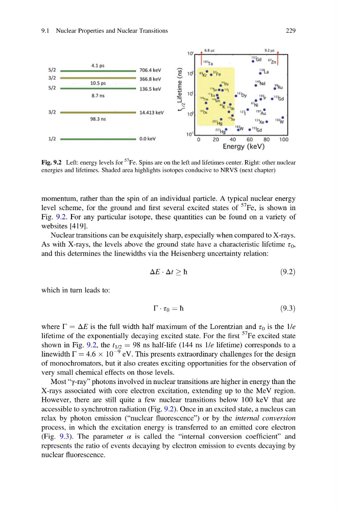
momentum, rather than the spin of an individual particle. A typical nuclear energy
level scheme, for the ground and first several excited states of
57 Fe, is shown in
Fig. 9.2. For any particular isotope, these quantities can be found on a variety of
websites [419].
Nuclear transitions can be exquisitely sharp, especially when compared to X-rays.
As with X-rays, the levels above the ground state have a characteristic lifetime τ 0 ,
and this determines the linewidths via the Heisenberg uncertainty relation:
ΔE Á Δt ! ħ
ð9:2Þ
which in turn leads to:
Γ Á τ 0 ¼ ħ
ð9:3Þ
where Γ ¼ ΔE is the full width half maximum of the Lorentzian and τ 0 is the 1/e
lifetime of the exponentially decaying excited state. For the first
57 Fe excited state
shown in Fig. 9.2, the t 1/2 ¼ 98 ns half-life (144 ns 1/e lifetime) corresponds to a
linewidth Γ ¼ 4.6 Â 10
À9 eV. This presents extraordinary challenges for the design
of monochromators, but it also creates exciting opportunities for the observation of
very small chemical effects on those levels.
Most “γ-ray” photons involved in nuclear transitions are higher in energy than the
X-rays associated with core electron excitation, extending up to the MeV region.
However, there are still quite a few nuclear transitions below 100 keV that are
accessible to synchrotron radiation (Fig. 9.2). Once in an excited state, a nucleus can
relax by photon emission (“nuclear fluorescence”) or by the internal conversion
process, in which the excitation energy is transferred to an emitted core electron
(Fig. 9.3). The parameter α is called the “internal conversion coefficient” and
represents the ratio of events decaying by electron emission to events decaying by
nuclear fluorescence.
Fig. 9.2 Left: energy levels for
57
Fe. Spins are on the left and lifetimes center. Right: other nuclear
energies and lifetimes. Shaded area highlights isotopes conducive to NRVS (next chapter)
9.1 Nuclear Properties and Nuclear Transitions
229
level scheme, for the ground and first several excited states of
57 Fe, is shown in
Fig. 9.2. For any particular isotope, these quantities can be found on a variety of
websites [419].
Nuclear transitions can be exquisitely sharp, especially when compared to X-rays.
As with X-rays, the levels above the ground state have a characteristic lifetime τ 0 ,
and this determines the linewidths via the Heisenberg uncertainty relation:
ΔE Á Δt ! ħ
ð9:2Þ
which in turn leads to:
Γ Á τ 0 ¼ ħ
ð9:3Þ
where Γ ¼ ΔE is the full width half maximum of the Lorentzian and τ 0 is the 1/e
lifetime of the exponentially decaying excited state. For the first
57 Fe excited state
shown in Fig. 9.2, the t 1/2 ¼ 98 ns half-life (144 ns 1/e lifetime) corresponds to a
linewidth Γ ¼ 4.6 Â 10
À9 eV. This presents extraordinary challenges for the design
of monochromators, but it also creates exciting opportunities for the observation of
very small chemical effects on those levels.
Most “γ-ray” photons involved in nuclear transitions are higher in energy than the
X-rays associated with core electron excitation, extending up to the MeV region.
However, there are still quite a few nuclear transitions below 100 keV that are
accessible to synchrotron radiation (Fig. 9.2). Once in an excited state, a nucleus can
relax by photon emission (“nuclear fluorescence”) or by the internal conversion
process, in which the excitation energy is transferred to an emitted core electron
(Fig. 9.3). The parameter α is called the “internal conversion coefficient” and
represents the ratio of events decaying by electron emission to events decaying by
nuclear fluorescence.
Fig. 9.2 Left: energy levels for
57
Fe. Spins are on the left and lifetimes center. Right: other nuclear
energies and lifetimes. Shaded area highlights isotopes conducive to NRVS (next chapter)
9.1 Nuclear Properties and Nuclear Transitions
229