

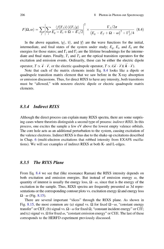
F Ω, ω
ð
Þ¼
X
f
X
i
f jT 2 ji
h
i ijT 1 jg
h
i
E g À E i þ Ω À iΓ i =2
2
Â
Γ f =2π
E g À E f þ Ω À ω
À
Á 2 þ Γ
2
f =4
ð8:4Þ
In the above equation, |gi, |ii, and |fi are the wave functions for the initial,
intermediate, and final states of the system under study; E g , E i , and E f are the
energies for those states; and Γ i and Γ f are the lifetime broadenings for the intermediate and final states. Finally, T 1 and T 2 are the optical transition operators for the
excitation and emission events. Ordinarily, these can be either the electric dipole
operator, T / e
! Á r
!
, or the electric quadrupole operator, T / i( e
! Á r
!
)( k
! Á r
! ).
Note that each of the matrix elements inside Eq. 8.4 looks like a dipole or
quadrupole transition matrix element that we saw before in the X-ray absorption
or emission discussions. Thus, for direct RIXS to have any intensity, both transitions
must be “allowed,” with nonzero electric dipole or electric quadrupole matrix
elements.
8.3.4 Indirect RIXS
Although the direct process can explain many RIXS spectra, there are some surprising cases where theorists distinguish a second type of process: indirect RIXS. In this
process, one excites the sample a few eV above the lowest empty valence orbitals.
The core hole acts as an additional perturbation to the system, causing excitation of
the valence electrons. Indirect RIXS is thus due to the shake-up excitations described
in Chap. 6 (multi-electron excitations that robbed intensity from EXAFS oscillations). We will see examples of indirect RIXS at both K- and L-edges.
8.3.5 The RIXS Plane
From Eq. 8.4 we see that (like resonance Raman) the RIXS intensity depends on
both excitation and emission energies. But instead of emission energy ω, the
quantity of interest is usually the energy loss, ΩÀω, since that is the energy of the
excitation in the sample. Thus, RIXS spectra are frequently presented as 3d representations or the corresponding contour plots vs. excitation energy Ω and energy loss
ΩÀω (Fig. 8.15).
There are several important “slices” through the RIXS plane. As shown in
Fig. 8.15, the most common are (a) signal vs. Ω for fixed ΩÀω, “constant energy
transfer” or CET; (b) signal vs. ΩÀω for fixed Ω, “constant incident energy” or CIT;
and (c) signal vs. Ω for fixed ω, “constant emission energy” or CEE. The last of these
corresponds to the HERFD experiment previously discussed.
206
8 Photon-in Photon-out Spectroscopy
ð
Þ¼
X
f
X
i
f jT 2 ji
h
i ijT 1 jg
h
i
E g À E i þ Ω À iΓ i =2
2
Â
Γ f =2π
E g À E f þ Ω À ω
À
Á 2 þ Γ
2
f =4
ð8:4Þ
In the above equation, |gi, |ii, and |fi are the wave functions for the initial,
intermediate, and final states of the system under study; E g , E i , and E f are the
energies for those states; and Γ i and Γ f are the lifetime broadenings for the intermediate and final states. Finally, T 1 and T 2 are the optical transition operators for the
excitation and emission events. Ordinarily, these can be either the electric dipole
operator, T / e
! Á r
!
, or the electric quadrupole operator, T / i( e
! Á r
!
)( k
! Á r
! ).
Note that each of the matrix elements inside Eq. 8.4 looks like a dipole or
quadrupole transition matrix element that we saw before in the X-ray absorption
or emission discussions. Thus, for direct RIXS to have any intensity, both transitions
must be “allowed,” with nonzero electric dipole or electric quadrupole matrix
elements.
8.3.4 Indirect RIXS
Although the direct process can explain many RIXS spectra, there are some surprising cases where theorists distinguish a second type of process: indirect RIXS. In this
process, one excites the sample a few eV above the lowest empty valence orbitals.
The core hole acts as an additional perturbation to the system, causing excitation of
the valence electrons. Indirect RIXS is thus due to the shake-up excitations described
in Chap. 6 (multi-electron excitations that robbed intensity from EXAFS oscillations). We will see examples of indirect RIXS at both K- and L-edges.
8.3.5 The RIXS Plane
From Eq. 8.4 we see that (like resonance Raman) the RIXS intensity depends on
both excitation and emission energies. But instead of emission energy ω, the
quantity of interest is usually the energy loss, ΩÀω, since that is the energy of the
excitation in the sample. Thus, RIXS spectra are frequently presented as 3d representations or the corresponding contour plots vs. excitation energy Ω and energy loss
ΩÀω (Fig. 8.15).
There are several important “slices” through the RIXS plane. As shown in
Fig. 8.15, the most common are (a) signal vs. Ω for fixed ΩÀω, “constant energy
transfer” or CET; (b) signal vs. ΩÀω for fixed Ω, “constant incident energy” or CIT;
and (c) signal vs. Ω for fixed ω, “constant emission energy” or CEE. The last of these
corresponds to the HERFD experiment previously discussed.
206
8 Photon-in Photon-out Spectroscopy