

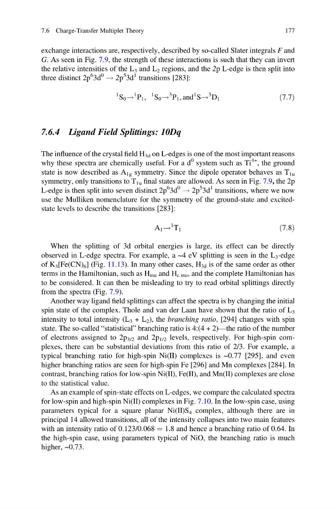
exchange interactions are, respectively, described by so-called Slater integrals F and
G. As seen in Fig. 7.9, the strength of these interactions is such that they can invert
the relative intensities of the L 3 and L 2 regions, and the 2p L-edge is then split into
three distinct 2p
6 3d
0
! 2p
5 3d
1 transitions [283]:
1 S 0 !
1 P 1 ,
1 S 0 !
3 P 1 , and
1 S!
3 D 1
ð7:7Þ
7.6.4 Ligand Field Splittings: 10Dq
The influence of the crystal field H 3d on L-edges is one of the most important reasons
why these spectra are chemically useful. For a d
0 system such as Ti
4+ , the ground
state is now described as A 1g symmetry. Since the dipole operator behaves as T 1u
symmetry, only transitions to T 1u final states are allowed. As seen in Fig. 7.9, the 2p
L-edge is then split into seven distinct 2p
6 3d
0
! 2p
5 3d
1 transitions, where we now
use the Mulliken nomenclature for the symmetry of the ground-state and excitedstate levels to describe the transitions [283]:
A 1 !
1 T 1
ð7:8Þ
When the splitting of 3d orbital energies is large, its effect can be directly
observed in L-edge spectra. For example, a ~4 eV splitting is seen in the L 3 -edge
of K 3 [Fe(CN) 6 ] (Fig. 11.13). In many other cases, H 3d is of the same order as other
terms in the Hamiltonian, such as H mu and H c:mu , and the complete Hamiltonian has
to be considered. It can then be misleading to try to read orbital splittings directly
from the spectra (Fig. 7.9).
Another way ligand field splittings can affect the spectra is by changing the initial
spin state of the complex. Thole and van der Laan have shown that the ratio of L 3
intensity to total intensity (L 3 + L 2 ), the branching ratio, [294] changes with spin
state. The so-called “statistical” branching ratio is 4:(4 + 2)—the ratio of the number
of electrons assigned to 2p 3/2 and 2p 1/2 levels, respectively. For high-spin complexes, there can be substantial deviations from this ratio of 2/3. For example, a
typical branching ratio for high-spin Ni(II) complexes is ~0.77 [295], and even
higher branching ratios are seen for high-spin Fe [296] and Mn complexes [284]. In
contrast, branching ratios for low-spin Ni(II), Fe(II), and Mn(II) complexes are close
to the statistical value.
As an example of spin-state effects on L-edges, we compare the calculated spectra
for low-spin and high-spin Ni(II) complexes in Fig. 7.10. In the low-spin case, using
parameters typical for a square planar Ni(II)S 4 complex, although there are in
principal 14 allowed transitions, all of the intensity collapses into two main features
with an intensity ratio of 0.123/0.068 ¼ 1.8 and hence a branching ratio of 0.64. In
the high-spin case, using parameters typical of NiO, the branching ratio is much
higher, ~0.73.
7.6 Charge-Transfer Multiplet Theory
177
G. As seen in Fig. 7.9, the strength of these interactions is such that they can invert
the relative intensities of the L 3 and L 2 regions, and the 2p L-edge is then split into
three distinct 2p
6 3d
0
! 2p
5 3d
1 transitions [283]:
1 S 0 !
1 P 1 ,
1 S 0 !
3 P 1 , and
1 S!
3 D 1
ð7:7Þ
7.6.4 Ligand Field Splittings: 10Dq
The influence of the crystal field H 3d on L-edges is one of the most important reasons
why these spectra are chemically useful. For a d
0 system such as Ti
4+ , the ground
state is now described as A 1g symmetry. Since the dipole operator behaves as T 1u
symmetry, only transitions to T 1u final states are allowed. As seen in Fig. 7.9, the 2p
L-edge is then split into seven distinct 2p
6 3d
0
! 2p
5 3d
1 transitions, where we now
use the Mulliken nomenclature for the symmetry of the ground-state and excitedstate levels to describe the transitions [283]:
A 1 !
1 T 1
ð7:8Þ
When the splitting of 3d orbital energies is large, its effect can be directly
observed in L-edge spectra. For example, a ~4 eV splitting is seen in the L 3 -edge
of K 3 [Fe(CN) 6 ] (Fig. 11.13). In many other cases, H 3d is of the same order as other
terms in the Hamiltonian, such as H mu and H c:mu , and the complete Hamiltonian has
to be considered. It can then be misleading to try to read orbital splittings directly
from the spectra (Fig. 7.9).
Another way ligand field splittings can affect the spectra is by changing the initial
spin state of the complex. Thole and van der Laan have shown that the ratio of L 3
intensity to total intensity (L 3 + L 2 ), the branching ratio, [294] changes with spin
state. The so-called “statistical” branching ratio is 4:(4 + 2)—the ratio of the number
of electrons assigned to 2p 3/2 and 2p 1/2 levels, respectively. For high-spin complexes, there can be substantial deviations from this ratio of 2/3. For example, a
typical branching ratio for high-spin Ni(II) complexes is ~0.77 [295], and even
higher branching ratios are seen for high-spin Fe [296] and Mn complexes [284]. In
contrast, branching ratios for low-spin Ni(II), Fe(II), and Mn(II) complexes are close
to the statistical value.
As an example of spin-state effects on L-edges, we compare the calculated spectra
for low-spin and high-spin Ni(II) complexes in Fig. 7.10. In the low-spin case, using
parameters typical for a square planar Ni(II)S 4 complex, although there are in
principal 14 allowed transitions, all of the intensity collapses into two main features
with an intensity ratio of 0.123/0.068 ¼ 1.8 and hence a branching ratio of 0.64. In
the high-spin case, using parameters typical of NiO, the branching ratio is much
higher, ~0.73.
7.6 Charge-Transfer Multiplet Theory
177