

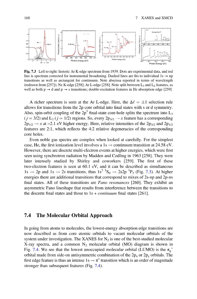
A richer spectrum is seen at the Ar L-edge. Here, the Δ‘ ¼ Æ1 selection rule
allows for transitions from the 2p core orbital into final states with s or d symmetry.
Also, spin-orbit coupling of the 2p
5
final-state core-hole splits the spectrum into L 3
( j ¼ 3/2) and L 2 ( j ¼ 1/2) regions. So, every 2p 3/2 ! x feature has a corresponding
2p 1/2 ! x at ~2.1 eV higher energy. Here, relative intensities of the 2p 3/2 and 2p 1/2
features are 2:1, which reflects the 4:2 relative degeneracies of the corresponding
core holes.
Even noble gas spectra are complex when looked at carefully. For the simplest
case, He, the first ionization level involves a 1s ! continuum transition at 24.58 eV.
However, there are discrete multi-electron events at higher energies, which were first
seen using synchrotron radiation by Madden and Codling in 1963 [258]. They were
later intensely studied by Shirley and coworkers [259]. The first of these
two-electron features is seen at 60.1 eV, and it can be described as simultaneous
1s ! 2p and 1s ! 2s transitions, thus 1s
2 1 S 0 ! 2s2p
1
P 1 (Fig. 7.3). At higher
energies there are additional transitions that correspond to mixes of 2s-np and 2p-ns
final states. All of these transitions are Fano resonances [260]. They exhibit an
asymmetric Fano lineshape that results from interference between the transitions to
the discrete final states and those to 1s + continuum final states [261].
7.4 The Molecular Orbital Approach
In going from atoms to molecules, the lowest-energy absorption edge transitions are
now described as from core atomic orbitals to vacant molecular orbitals of the
system under investigation. The XANES for N 2 is one of the best-studied molecular
X-ray spectra, and a common N 2 molecular orbital (MO) diagram is shown in
Fig. 7.4. We see that the lowest unoccupied molecular orbital (LUMO) is the π g
Ã
orbital made from side-on antisymmetric combination of the 2p x or 2p y orbitals. The
first edge feature is thus an intense 1s ! π
à transition which is an order of magnitude
stronger than subsequent features (Fig. 7.4).
Fig. 7.3 Left to right: historic Ar K-edge spectrum from 1939. Dots are experimental data, and red
line is spectrum corrected for instrumental broadening. Dashed lines are fits to individual 1s → np
transitions as well as arctangent for continuum. Note abscissa reported in terms of wavelength
(redrawn from [257]); Ne K-edge [258]; Ar L-edge [258]. Note split between L 3 and L 2 features, as
well as both p → d and p → s transitions; double-excitation features in He absorption edge [259]
168
7 XANES and XMCD
allows for transitions from the 2p core orbital into final states with s or d symmetry.
Also, spin-orbit coupling of the 2p
5
final-state core-hole splits the spectrum into L 3
( j ¼ 3/2) and L 2 ( j ¼ 1/2) regions. So, every 2p 3/2 ! x feature has a corresponding
2p 1/2 ! x at ~2.1 eV higher energy. Here, relative intensities of the 2p 3/2 and 2p 1/2
features are 2:1, which reflects the 4:2 relative degeneracies of the corresponding
core holes.
Even noble gas spectra are complex when looked at carefully. For the simplest
case, He, the first ionization level involves a 1s ! continuum transition at 24.58 eV.
However, there are discrete multi-electron events at higher energies, which were first
seen using synchrotron radiation by Madden and Codling in 1963 [258]. They were
later intensely studied by Shirley and coworkers [259]. The first of these
two-electron features is seen at 60.1 eV, and it can be described as simultaneous
1s ! 2p and 1s ! 2s transitions, thus 1s
2 1 S 0 ! 2s2p
1
P 1 (Fig. 7.3). At higher
energies there are additional transitions that correspond to mixes of 2s-np and 2p-ns
final states. All of these transitions are Fano resonances [260]. They exhibit an
asymmetric Fano lineshape that results from interference between the transitions to
the discrete final states and those to 1s + continuum final states [261].
7.4 The Molecular Orbital Approach
In going from atoms to molecules, the lowest-energy absorption edge transitions are
now described as from core atomic orbitals to vacant molecular orbitals of the
system under investigation. The XANES for N 2 is one of the best-studied molecular
X-ray spectra, and a common N 2 molecular orbital (MO) diagram is shown in
Fig. 7.4. We see that the lowest unoccupied molecular orbital (LUMO) is the π g
Ã
orbital made from side-on antisymmetric combination of the 2p x or 2p y orbitals. The
first edge feature is thus an intense 1s ! π
à transition which is an order of magnitude
stronger than subsequent features (Fig. 7.4).
Fig. 7.3 Left to right: historic Ar K-edge spectrum from 1939. Dots are experimental data, and red
line is spectrum corrected for instrumental broadening. Dashed lines are fits to individual 1s → np
transitions as well as arctangent for continuum. Note abscissa reported in terms of wavelength
(redrawn from [257]); Ne K-edge [258]; Ar L-edge [258]. Note split between L 3 and L 2 features, as
well as both p → d and p → s transitions; double-excitation features in He absorption edge [259]
168
7 XANES and XMCD